Geometry of Neural Activations, Part 1: High-Dimensional Geometry and Compressed Sensing
Published:
Part Title Core question 1 High-Dimensional Geometry and Compressed Sensing How can infinitely many “directions” fit in a finite space, and when is a sparse code recoverable? 2 Sparse Autoencoders and Superposition How do we actuallyfind those features in a trained model, and what does their existence prove? 3 Steering, Linear Structure, and Feature Manifolds If we find a feature, how do we prove it is causal — and what does it miss? Part 1 is the mathematical foundation. Everything in Parts 2 and 3 is an engineering or empirical instantiation of the geometry developed here.
Table of Contents
- What Is a Neural Activation?
- 1.1 The residual stream
- 1.2 The representational bottleneck
- 1.3 Two escape routes: geometry and sparsity
- 1.4 Notation
- High-Dimensional Geometry
- 2.1 The unit sphere and spherical caps
- 2.2 A cap-volume bound
- 2.3 Random vectors are nearly orthogonal
- 2.4 Large nearly-orthogonal packings exist
- 2.5 Worked numbers: how many directions fit in 2000 dimensions?
- Sparsity and Compressed Sensing
- 3.1 Sparse vectors and the set $\Sigma_s$
- 3.2 Generic injectivity on sparse vectors
- 3.3 The restricted isometry property
- 3.4 Gaussian random matrices satisfy RIP
- 3.5 Consequences of RIP — injectivity, inner-product preservation, exact recovery by basis pursuit
- 3.6 Worked numbers: how many measurements do we need?
- 3.7 The chain so far
- Part 1 Takeaways References for Part 1
1. What Is a Neural Activation?
Everything in this series is about vectors and the geometry between them. Before we can ask geometric questions about activations, we need to know precisely what an activation is, where it lives, and why anyone believes its geometry matters.
1.1 The residual stream
A transformer language model processes text one token at a time. Each token is mapped to a vector; each layer reads that vector, computes an update, and writes the update back to the same place. The shared “place” is called the residual stream.
A standard pre-norm block has the form
\[x^{(\ell+1)} = x^{(\ell)} + \operatorname{Attn}\!\left(x^{(\ell)}\right) + \operatorname{MLP}\!\left(x^{(\ell)}\right),\]where $x^{(\ell)}\in\mathbb R^{d}$ is the residual-stream vector at layer $\ell$ and $d$ is the model width (hidden size). The same $d$-dimensional vector carries the token identity, position information, syntactic state, semantic content, factual associations, and the model’s current “task state” — all at once, all mixed together.

The picture above is a standard transformer block. The important feature for us is the skip connection structure: attention and MLP do not replace the residual stream, they add to it. Every write is an addition of some vector to a running total. This is why “superposition” (Part 2) is even a sensible idea — the residual stream is literally an additive accumulator, and each concept that the model tracks contributes a direction to that accumulator.
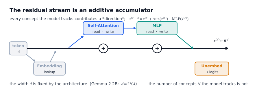
Figure 1.1 — The residual stream as an additive accumulator. Attention and MLP read the stream and write a vector back into it; the stream’s width $d$ is fixed by the architecture, while the number of concepts $N$ the model tracks is not.
What we mean by “an activation”
Throughout this series, a single activation is a vector
\[x\in\mathbb R^{d},\]read off the residual stream at a chosen site (e.g. the output of layer $\ell$ at a given token position). A model with $L$ layers processes a sequence of $T$ tokens by producing a whole trajectory of such vectors:
\[x_t^{(\ell)}\in\mathbb R^{d}, \qquad t=1,\dots,T,\quad \ell=1,\dots,L.\]When we collect a training corpus of activations for an autoencoder, we get a point cloud ${x_1,\dots,x_n}\subseteq\mathbb R^d$ sampled from the model’s activity.
1.2 The representational bottleneck
The width $d$ is fixed at training time. For reference, Gemma 2 2B has
\[d=2304,\]and a vocabulary of $256{,}000$ tokens.
But the number of things a language model tracks is not bounded by $d$. A model must distinguish tokens, but it must also represent syntactic category, tense, number, named entities, factual associations, discourse state, sentiment, register, the identity of the user, the current task, and an open-ended supply of domain concepts. Call the number of such conceptual features $N$. Empirically we expect
\[N \gg d.\]So we have a genuine representational bottleneck: a $d$-dimensional vector cannot hold $N>d$ mutually orthogonal, independently readable features.
The central representational hypothesis of this series is that the model does not need mutually orthogonal features. Instead, the residual stream is (approximately) a sparse combination of many directions:
\[\boxed{ x \;\approx\; \sum_{i=1}^{N} a_i\, w_i, \qquad a_i\ge 0, \qquad \|w_i\|_2=1, \qquad \|a\|_0 \ll N. }\]where:
- $w_i\in\mathbb R^{d}$ is a unit-norm feature direction;
- $a_i\ge 0$ is the activation of feature $i$ on this input;
- $N$ is the number of features the model has available;
- only a small number of the $a_i$ are nonzero.
Note this is an overcomplete representation: the dictionary ${w_i}$ has more atoms than the space has dimensions. The “activation” in the title of this series has a precise meaning here — it is a coefficient in an overcomplete expansion, and the interesting question is whether that expansion is readable (unique, stable, interpretable).
1.3 Two escape routes: geometry and sparsity
Why can’t the model just use $d$ orthogonal directions? It can — and it does, at the level of individual neurons. The escape from the bottleneck requires two ingredients, and neither is sufficient alone.
Route 1: Geometry — there is more room than dimension suggests.
In $\mathbb R^d$ you cannot have more than $d$ mutually orthogonal unit vectors. But you can have exponentially many vectors that are merely “nearly orthogonal”, i.e. whose pairwise inner products are small. For $d=2000$ we will prove in §2.4 that there exist on the order of $10^{13}$ unit vectors with all pairwise inner products at most $\cos 80^\circ \approx 0.17$. The space is far roomier than “dimension $d$” suggests. Cost: the directions are not perfectly distinguishable.
Route 2: Sparsity — not all features are active at once.
Even if the directions are only approximately orthogonal, a given input activates only a small number of them. If at most $s$ features are active, and $s$ is much smaller than $d$, then the active set occupies a low-dimensional subspace that may be recoverable from a generic projection. This is exactly the setting of compressed sensing.
The two routes interlock:
- without sparsity, near-orthogonality is not enough (an arbitrary $N$-vector in $\mathbb R^d$ is not recoverable from a $d$-dimensional measurement);
- without near-orthogonality, sparsity is not enough (if the features were collinear, no method could separate them).
The entire mathematical content of Part 1 is the rigorous version of this claim: high-dimensional near-orthogonality plus sparsity allows many features to coexist in a low-dimensional activation space.
1.4 Notation
We use the following notation consistently across all three parts.
Spaces and sets
- $\mathbb R^d$, $\mathbb R^N$: the $d$-dimensional activation space and the $N$-dimensional feature space.
- $\mathbb S^{d-1}={x\in\mathbb R^d:|x|_2=1}$: the unit sphere.
- $B(c,r)={x\in\mathbb R^d:|x-c|_2\le r}$: the closed Euclidean ball.
- $\Sigma_s={a\in\mathbb R^N:|a|_0\le s}$: the set of $s$-sparse vectors.
- $E_S={a\in\mathbb R^N:\operatorname{supp}(a)\subseteq S}$: the coordinate subspace indexed by $S\subseteq[N]$.
Norms and inner products
- $\langle x,y\rangle=x^\top y$.
$|x|_2=|x|$; $|x|_1=\sum_i x_i $; $|x|_0=#{i:x_i\neq 0}$. - $\operatorname{supp}(x)={i:x_i\neq0}$; $e_i$ is the $i$-th standard basis vector of $\mathbb R^N$.
Compressed sensing (Part 1, Chapter 3)
- $A\in\mathbb R^{d\times N}$: the measurement matrix.
- $a\in\mathbb R^N$: the sparse coefficient vector; $b=Aa\in\mathbb R^d$: the measurement.
Sparse autoencoders (Part 2)
- $x\in\mathbb R^d$: an activation; $f(x)\in\mathbb R^N_{\ge0}$: the sparse code.
- $W_{\mathrm{dec}}\in\mathbb R^{d\times N}$: the decoder (dictionary); $w_i=W_{\mathrm{dec}}e_i\in\mathbb R^d$: the $i$-th feature direction.
- $b_{\mathrm{pre}}\in\mathbb R^d$: the pre-activation bias.
- $\operatorname{ReLU}(z)=\max(z,0)$, applied coordinatewise.
Measure
- $\sigma_{d-1}(\cdot)$: surface area measure on $\mathbb S^{d-1}$ (unnormalized). Hence $\operatorname{Vol}d(B(0,1))=\frac1d\,\sigma{d-1}(\mathbb S^{d-1})$.
2. High-Dimensional Geometry
Everything we need about “how many directions can we cram into $\mathbb R^d$” comes from estimating the size of a spherical cap.
2.1 The unit sphere and spherical caps
Fix a direction $u\in\mathbb S^{d-1}$. For $t\in[0,1]$ define the spherical cap
\[\operatorname{cap}(u,t) = \left\{ v\in\mathbb S^{d-1} : \langle u,v\rangle \ge t \right\}.\]Equivalently, the set of directions within angle $\arccos(t)$ of $u$.
Its normalized size is
\[p_d(t) = \frac{\sigma_{d-1}\!\left(\operatorname{cap}(u,t)\right)} {\sigma_{d-1}\!\left(\mathbb S^{d-1}\right)} \in[0,1].\]By rotational symmetry of the sphere, $p_d(t)$ depends only on $d$ and $t$, not on $u$. Intuitively, $p_d(t)$ is the probability that a uniformly random unit vector $v$ satisfies $\langle u,v\rangle\ge t$ — i.e. that $v$ is “close enough” to $u$ to be confused with it.
The single most important fact in this chapter is that $p_d(t)$ shrinks exponentially in $d$, so a random direction in high dimension is very far from any fixed direction.
2.2 A cap-volume bound
Lemma 1 (cap bound). For every $d\ge 2$ and every $0\le t\le 1/\sqrt2$,
\[p_d(t) \;\le\; (1-t^2)^{d/2} \;\le\; e^{-dt^2/2}.\]Proof. Identify the cap with the solid cone it spans from the origin:
\[C(u,t) = \left\{ \rho v : 0\le\rho\le 1,\ v\in\operatorname{cap}(u,t) \right\}.\]A cone over a set of $(d-1)$-dimensional surface measure $\sigma$ has $d$-dimensional volume $\sigma/d$, so
\[\operatorname{Vol}_d(C(u,t)) = \frac1d\,\sigma_{d-1}\!\left(\operatorname{cap}(u,t)\right), \qquad \operatorname{Vol}_d(B(0,1)) = \frac1d\,\sigma_{d-1}\!\left(\mathbb S^{d-1}\right).\]Hence
\[p_d(t) = \frac{\operatorname{Vol}_d(C(u,t))} {\operatorname{Vol}_d(B(0,1))}.\]Set $q=tu$, the centre of the hyperplane that cuts off the cap. For $v\in\operatorname{cap}(u,t)$ we have $\langle u,v\rangle\ge t$, so
\[\begin{aligned} \|v-q\|_2^2 &=\|v-tu\|_2^2\\ &=\|v\|_2^2-2t\langle u,v\rangle+t^2\|u\|_2^2\\ &=1-2t\langle u,v\rangle+t^2\\ &\le 1-2t^2+t^2\\ &=1-t^2. \end{aligned}\]Therefore $\operatorname{cap}(u,t)\subseteq B(q,\sqrt{1-t^2})$.
Now take a cone point $x=\rho v$ with $0\le\rho\le1$ and $v\in\operatorname{cap}(u,t)$. By convexity of the norm,
\[\|x-q\|_2 = \|\rho v-(1-\rho)q\|_2 \le \rho\|v-q\|_2+(1-\rho)\|q\|_2 \le \rho\sqrt{1-t^2}+(1-\rho)t.\]If $t\le 1/\sqrt2$ then $t\le\sqrt{1-t^2}$, so the right-hand side is at most $\sqrt{1-t^2}$. Thus
\[C(u,t)\subseteq B\!\left(tu,\sqrt{1-t^2}\right).\]Taking $d$-dimensional volumes and using translation invariance and scaling of Lebesgue measure,
\[p_d(t) \le \frac{\operatorname{Vol}_d\!\left(B(tu,\sqrt{1-t^2})\right)} {\operatorname{Vol}_d(B(0,1))} = (1-t^2)^{d/2}.\]Finally $1-x\le e^{-x}$ with $x=t^2$ gives
\[(1-t^2)^{d/2} = \left(1-t^2\right)^{d/2} \le \left(e^{-t^2}\right)^{d/2} = e^{-dt^2/2}. \qquad\blacksquare\]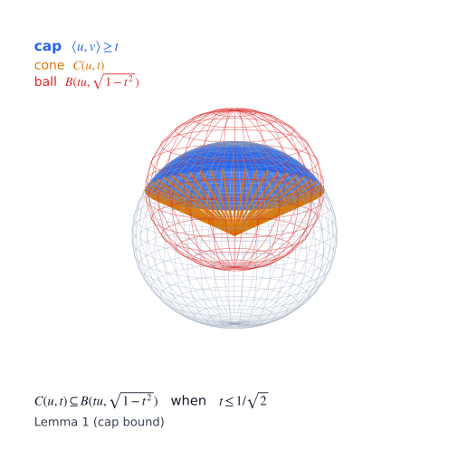
Figure 2.1 — The geometry behind Lemma 1. The spherical cap $\operatorname{cap}(u,t)$ (blue) sits on the unit sphere; the cone $C(u,t)$ it spans (amber) is contained in the ball $B(tu,\sqrt{1-t^2})$ (red) as long as $t\le 1/\sqrt2$. Taking volumes converts this inclusion into the cap bound.
Remark (the range of validity matters). Two things are true and are often conflated:
- The exponential bound $p_d(t)\le e^{-dt^2/2}$ holds for all $t\in[0,1]$ — this is the standard spherical-cap estimate and is what one should quote.
- The polynomial bound $p_d(t)\le(1-t^2)^{d/2}$ is what the cone-containment proof above delivers, and that proof requires $t\le 1/\sqrt2$.
The polynomial bound is not valid for all $t$. For example, in $d=2$ the cap is an arc and $p_2(t)=\arccos(t)/\pi$; at $t=0.99$ we get
\[p_2(0.99)\approx 0.04505 \;>\; (1-0.99^2)^{1}=0.0199.\]So the “sharper” form is not a uniform sharpening — it is a different statement with a smaller range of validity. The exponential form dominates it in the regime we care about ($t$ small, $d$ large), which is why the lemma is stated the way it is.
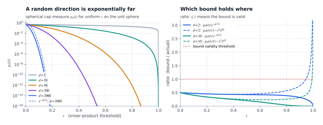
Figure 2.2 — Left: the cap measure $p_d(t)$ collapses exponentially as the dimension grows, so a random direction in high dimension is essentially orthogonal to every fixed direction. Right: the ratio of each bound to the true cap measure. The exponential bound $e^{-dt^2/2}$ stays below $1$ (valid) for every $t\in[0,1]$; the polynomial bound $(1-t^2)^{d/2}$ crosses above $1$ for $t$ close to $1$ in small dimension.
2.3 Random vectors are nearly orthogonal
Lemma 2 (random near-orthogonality). Let $v_1,\dots,v_N$ be independent and uniformly distributed on $\mathbb S^{d-1}$. For $0\le t\le 1/\sqrt2$,
\[\mathbb P\!\left( \max_{1\le i<j\le N}\langle v_i,v_j\rangle>t \right) \le \binom N2 e^{-dt^2/2} \le \frac{N^2}{2}e^{-dt^2/2}.\]Proof. Fix $i<j$. Conditional on $v_i$, the vector $v_j$ is still uniform on $\mathbb S^{d-1}$, so
\[\mathbb P\!\left(\langle v_i,v_j\rangle>t \mid v_i\right)=p_d(t)\le e^{-dt^2/2}.\]Averaging over $v_i$ and applying the union bound over the $\binom N2$ unordered pairs,
\[\begin{aligned} \mathbb P\!\left(\exists\, i<j:\ \langle v_i,v_j\rangle>t\right) &\le \sum_{1\le i<j\le N}\mathbb P\!\left(\langle v_i,v_j\rangle>t\right)\\ &\le \binom N2 e^{-dt^2/2}\\ &\le \frac{N^2}{2}e^{-dt^2/2}. \end{aligned} \qquad\blacksquare\]Corollary 3. If
\[N\le e^{dt^2/4},\]then with probability at least $1/2$ every pair satisfies $\langle v_i,v_j\rangle\le t$.
Proof. By Lemma 2 it suffices that
\[\frac{N^2}{2}e^{-dt^2/2}\le\frac12 \iff N^2\le e^{dt^2/2} \iff N\le e^{dt^2/4}. \qquad\blacksquare\]Interpretation. For $d=2000$ and $t=\cos 80^\circ\approx 0.1736$ we have $dt^2/2\approx 30.15$, so $e^{dt^2/4}\approx 3.5\times 10^{6}$ random directions can be drawn while keeping all pairwise angles at least $80^\circ$ with probability at least $1/2$. Randomness is a blunt instrument: the next section shows that a deliberate construction does far better.
2.4 Large nearly-orthogonal packings exist
Lemma 2 is an average-case statement (“random vectors are fine”). What we actually need for superposition is an existence statement: there is a configuration of exponentially many directions with controlled mutual overlap.
Proposition 4 (probabilistic packing). For every $0<t\le 1/\sqrt2$ there exists a finite set
\[V=\{v_1,\dots,v_M\}\subseteq\mathbb S^{d-1}\]such that
\[M\;\ge\;\frac{3}{8}\,e^{dt^2/2} \qquad\text{and}\qquad \langle v_i,v_j\rangle\le t \ \ \text{for all } i\ne j.\]Proof. Write $p=p_d(t)$ and draw
\[n=\left\lceil\frac{1}{2p}\right\rceil\]independent uniform points $u_1,\dots,u_n$ on $\mathbb S^{d-1}$. Call a pair $(i,j)$ bad if $\langle u_i,u_j\rangle>t$. The expected number of bad pairs is
\[\mathbb E[\#\text{bad}] = \binom n2 p \le \frac{n^2}{2}p.\]Now repeatedly select a bad pair and delete one of its two endpoints, until no bad pair remains. At most one point is deleted per bad pair, so the surviving set $V$ satisfies
\[|V|\ \ge\ n-\#\text{bad}.\]Taking expectations, some realization satisfies
\[|V|\ \ge\ n-\frac{n^2}{2}p.\]To evaluate this, write $n=\frac{1}{2p}+r$ with $0\le r<1$. Then
\[\begin{aligned} n-\frac{n^2}{2}p &= \frac{1}{2p}+r-\frac p2\left(\frac{1}{2p}+r\right)^2\\ &= \frac{1}{2p}+r-\frac{1}{8p}-\frac r2-\frac{pr^2}{2}\\ &= \frac{3}{8p}+\frac r2\left(1-pr\right)\\ &\ge \frac{3}{8p}, \end{aligned}\]since $pr<1$. Hence $M\ge \frac{3}{8p}$. Finally, Lemma 1 gives $p=p_d(t)\le e^{-dt^2/2}$, so
\[M\ \ge\ \frac{3}{8p}\ \ge\ \frac38\,e^{dt^2/2}. \qquad\blacksquare\]Interpretation. The bound is exponential in $d$. This is the geometric room that makes overcomplete feature dictionaries plausible at all: the residual stream of a 2000-dimensional model has exponentially more “almost-orthogonal slots” than a naive dimension count suggests. The price of using those slots is that the slots are not perfectly independent — which is precisely what Part 2 (superposition) and Part 3 (interference between features) are about.
2.5 Worked numbers: how many directions fit in 2000 dimensions?
Let
\[d=2000, \qquad \theta=80^\circ, \qquad t=\cos 80^\circ\approx 0.17365, \qquad t^2\approx 0.030154.\]Then
\[\frac{dt^2}{2} = \frac{2000\times 0.030154}{2} \approx 30.15, \qquad e^{dt^2/2}\approx 1.246\times 10^{13}.\]Existence (Proposition 4). There is a set of directions with all pairwise angles $\ge 80^\circ$ of size at least
\[M\ \ge\ \frac38\times 1.246\times10^{13}\ \approx\ 4.7\times10^{12}.\]So on the order of $10^{13}$ such directions exist.
Random construction (Lemma 2). To make the probability that any pair violates the $80^\circ$ separation smaller than $1\%$ we need
\[\frac{N^2}{2}e^{-30.15}<0.01 \iff N^2<0.02\,e^{30.15} \iff N<\sqrt{0.02}\times e^{15.07}\approx 5.0\times10^{5}.\]So roughly $5\times 10^{5}$ random directions can be chosen with $99\%$ confidence, while a deliberately constructed set achieves seven orders of magnitude more. Randomness is not the resource — the high-dimensional geometry is.
Summary. In $d=2000$ dimensions the sphere supports astronomically many directions that are mutually “close to orthogonal”. A $d$-dimensional residual stream is nowhere near as constrained as “$d$ features”.
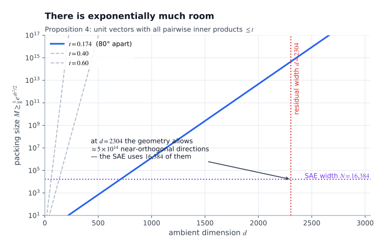
Figure 2.3 — The packing size grows as $e^{dt^2/2}$. At the operating point of a 2304-dimensional residual stream, the geometry permits on the order of $10^{14}$ mutually 80°-separated directions; a Gemma Scope SAE of width 16,384 uses a vanishingly small fraction of them. The geometry is not the binding constraint on feature count — sparsity and identifiability are.
3. Sparsity and Compressed Sensing
Geometry tells us there is room. It does not tell us the features are readable. That is the job of sparsity, and the formal language for it is compressed sensing.
3.1 Sparse vectors and the set $\Sigma_s$
A vector $a\in\mathbb R^N$ is $s$-sparse if
\[\|a\|_0\le s.\]The set of all $s$-sparse vectors is
\[\Sigma_s = \{a\in\mathbb R^N:\|a\|_0\le s\} = \bigcup_{\substack{S\subseteq[N]\\|S|\le s}} E_S.\]For $0<s<N$ this is not a linear subspace: it is a finite union of coordinate subspaces, one for each candidate support. This non-convexity is the source of essentially all the difficulty — and of the $\ell_1$ convex relaxation that eventually solves it.
Note the geometry of $\Sigma_s$: it is a union of $\binom Ns$-many $s$-dimensional linear pieces. The number of “candidate supports” is the combinatorial price of not knowing which features are active, and it will reappear in the RIP sample complexity (§3.4) as the term $k\log(N/k)$.
3.2 Generic injectivity on sparse vectors
Let $A\in\mathbb R^{d\times N}$ be a linear map from feature space to activation space. We ask the weakest possible question: when are distinct sparse feature vectors guaranteed to have distinct images?
Lemma 5 (generic injectivity on $\Sigma_s$). Let $A\in\mathbb R^{d\times N}$ be generic (i.e. outside a proper algebraic subset of the matrix space). If
\[d\ge 2s,\]then $A$ is injective on $\Sigma_s$. Equivalently,
\[\ker(A)\cap\Sigma_{2s}=\{0\}.\]Proof. Suppose $a,b\in\Sigma_s$ with $Aa=Ab$, and put $h=a-b$. Then
\[Ah=0, \qquad \|h\|_0\le \|a\|_0+\|b\|_0\le 2s,\]so $h\in\ker(A)\cap\Sigma_{2s}$. It remains to show this intersection is trivial.
Write
\[\Sigma_{2s}=\bigcup_{\substack{T\subseteq[N]\\|T|=2s}} E_T\]and fix one such $T$. For generic $A$ we have $\dim\ker(A)=N-d$, and generic transversality gives
\[\dim\bigl(\ker(A)\cap E_T\bigr) = \max\{0,\ \dim\ker(A)+\dim E_T-N\} = \max\{0,\ (N-d)+2s-N\} = \max\{0,\ 2s-d\}.\]Since $d\ge 2s$, this dimension is $0$, so $\ker(A)\cap E_T={0}$ for every $T$, whence $\ker(A)\cap\Sigma_{2s}={0}$. Therefore $h=0$ and $a=b$. $\qquad\blacksquare$
Remark (the threshold is sharp). The condition $d\ge 2s$ is exactly right, and it is worth seeing why. The quantity that governs everything is the spark of $A$, i.e. the size of the smallest linearly dependent set of columns:
\[\operatorname{spark}(A)=\min\{|T|:\ A_T \text{ is column-rank deficient}\}.\]A nonzero kernel vector with support of size $2s$ exists iff $\operatorname{spark}(A)\le 2s$. For a generic $d\times N$ matrix with $N>d$ we have $\operatorname{spark}(A)=d+1$ (any $d$ columns are generically independent; any $d+1$ are dependent). Hence
\[\ker(A)\cap\Sigma_{2s}=\{0\} \iff \operatorname{spark}(A)>2s \iff d+1>2s \iff d\ge 2s.\]Equivalently: to have $N>d$ columns, some $d+1$ of them must be dependent, and that dependence is generically spread over all $d+1$ of them.
3.3 The restricted isometry property
Injectivity tells us distinctness but says nothing about geometry: it does not tell us that distances, angles or inner products are preserved, and it says nothing about whether we can compute the sparse code. The right notion is quantitative.
Definition 6 (restricted isometry property, RIP). A matrix $A\in\mathbb R^{d\times N}$ satisfies the $(k,\delta)$-RIP if for every $a\in\Sigma_k$,
\[(1-\delta)\|a\|_2^2 \;\le\; \|Aa\|_2^2 \;\le\; (1+\delta)\|a\|_2^2.\]Equivalently,
\[\left|\|Aa\|_2^2-\|a\|_2^2\right|\le \delta\|a\|_2^2 \qquad\text{for all }a\in\Sigma_k.\]The smallest such $\delta$ is the restricted isometry constant $\delta_k(A)$.
Interpretation. RIP says: on the set of $k$-sparse vectors, $A$ is approximately an isometry. It does not matter what $A$ does to the rest of $\mathbb R^N$ — it may stretch, squash and scramble dense vectors arbitrarily. It only has to behave on the sparse ones. This is precisely the property we want when we believe the network’s activations are sparse combinations of features.
Two immediate sanity checks:
- $A$ satisfies the $(2k,\delta)$-RIP for some $\delta<1$ iff $A$ is injective on $\Sigma_k$ (Proposition 8 below). Injectivity is the qualitative shadow of RIP; RIP is the quantitative version.
- RIP is monotone: $(k,\delta)$-RIP implies $(k’,\delta)$-RIP for $k’\le k$.
3.4 Gaussian random matrices satisfy RIP
Theorem 7 (Gaussian RIP). Let $G\in\mathbb R^{d\times N}$ have i.i.d. standard Gaussian entries and set
\[A=\frac{1}{\sqrt d}G.\]Fix $1\le k\le N$, $0<\delta<1$, and failure probability $0<\eta<1$. There is a universal constant $C>0$ such that if
\[\boxed{ d\ \ge\ C\,\delta^{-2}\left(k\log\frac Nk+\log\frac1\eta\right), }\]then $A$ satisfies the $(k,\delta)$-RIP with probability at least $1-\eta$.
| Proof sketch. Fix a support $S\subseteq[N]$ with $ | S | =k$. The restricted matrix $A_S\in\mathbb R^{d\times k}$ has i.i.d. $N(0,1/d)$ entries. For a fixed unit vector $x\in\mathbb S^{k-1}$, |
where $g_1,\dots,g_d$ are independent standard Gaussian vectors in $\mathbb R^k$. Each $\langle g_r,x\rangle$ is standard Gaussian, so $|A_Sx|_2^2$ is the average of $d$ independent $\chi^2_1$ variables. Concentration of sub-Gaussian quadratic forms gives
\[\mathbb P\!\left(\left|\|A_Sx\|_2^2-1\right|>\delta\right)\le 2e^{-c d\delta^2}\]for a universal $c>0$.
To make this uniform over all $x\in\mathbb S^{k-1}$, cover the sphere by an $\varepsilon$-net $\mathcal N$ with
\[|\mathcal N|\le\left(1+\frac2\varepsilon\right)^k.\]A standard net argument (control on the net plus a Lipschitz bound on the quadratic form) turns pointwise concentration into uniform control:
\[\mathbb P\!\left( \sup_{x\in\mathbb S^{k-1}} \left|\|A_Sx\|_2^2-1\right|>\delta \right) \le \exp\!\left(-c' d\delta^2+C'k\right).\]Finally, union-bound over the $\binom Nk$ candidate supports:
\[\mathbb P(\text{RIP fails}) \le \binom Nk \exp\!\left(-c'd\delta^2+C'k\right).\]Using $\binom Nk\le\left(\frac{eN}{k}\right)^k$, it suffices that
\[k\log\frac{eN}{k}-c'd\delta^2+C'k+\log\frac1\eta\le 0,\]which is implied by the stated condition on $d$. $\qquad\blacksquare$
This concentration-plus-covering strategy is the standard elementary proof of RIP for sub-Gaussian random matrices (Baraniuk–Davenport–DeVore–Wakin).
Interpretation of the sample complexity. The term
\[k\log\frac Nk\]is the combinatorial price of not knowing which $k$ coordinates are active: there are $\binom Nk\approx(eN/k)^k$ candidate supports, and $d$ must be large enough to control all of them simultaneously. The term $\log(1/\eta)$ controls the failure probability. Note carefully that $\eta$ is the failure probability and $\delta$ is the distortion; confusing the two is a common error.
The key asymptotic fact: $d$ must scale like $s\log(N/s)$, not like $N$. This is the entire reason compressed sensing works, and it is the reason the residual stream does not need to be as wide as the number of features.
3.5 Consequences of RIP
3.5.1 Injectivity
Proposition 8. If $A$ satisfies the $(2s,\delta)$-RIP with $\delta<1$, then $A$ is injective on $\Sigma_s$.
Proof. Suppose $a,b\in\Sigma_s$ with $Aa=Ab$ and set $h=a-b$. Then $|h|0\le 2s$, so $h\in\Sigma{2s}$, and $Ah=0$. By RIP,
\[(1-\delta)\|h\|_2^2\le\|Ah\|_2^2=0.\]Since $1-\delta>0$, $|h|_2=0$, hence $h=0$ and $a=b$. $\qquad\blacksquare$
3.5.2 Inner-product preservation
Lemma 9 (geometric stability). If $A$ satisfies the $(2s,\delta)$-RIP then for all $a,b\in\Sigma_s$,
\[\left| \langle Aa,Ab\rangle-\langle a,b\rangle \right| \le \delta\,\|a\|_2\,\|b\|_2.\]In particular, writing $w_i=Ae_i$ for the $i$-th column of $A$, for every $a\in\Sigma_s$,
\[\left|\langle Aa,w_i\rangle-a_i\right|\le\delta\,\|a\|_2.\]Proof. By the polarization identity,
\[\langle a,b\rangle=\frac14\left(\|a+b\|_2^2-\|a-b\|_2^2\right),\]and likewise for $Aa,Ab$. Since $a,b\in\Sigma_s$, both $a+b$ and $a-b$ lie in $\Sigma_{2s}$, so RIP applies to each:
\[\left|\|A(a\pm b)\|_2^2-\|a\pm b\|_2^2\right|\le\delta\|a\pm b\|_2^2.\]Therefore
\[\begin{aligned} \left|\langle Aa,Ab\rangle-\langle a,b\rangle\right| &\le \frac14\left(\delta\|a+b\|_2^2+\delta\|a-b\|_2^2\right)\\ &= \frac{\delta}{4}\left(2\|a\|_2^2+2\|b\|_2^2\right) \qquad \text{(parallelogram identity)}\\ &= \frac{\delta}{2}\left(\|a\|_2^2+\|b\|_2^2\right)\\ &\le \delta\,\|a\|_2\|b\|_2 \qquad \text{(AM–GM)}. \end{aligned}\]Finally take $b=e_i$: then $Ab=w_i$, $|b|_2=1$, and $\langle a,b\rangle=a_i$, giving the readout bound. $\qquad\blacksquare$
Interpretation. If the compressed activation is $b=Aa$, then the $i$-th sparse coefficient can be approximately read off by projecting onto the $i$-th dictionary column:
\[a_i\;\approx\;\langle b,w_i\rangle.\]This is the “dictionary is self-consistent” property that a learned SAE must also satisfy: a feature’s activation should be recoverable by projecting the activation onto that feature’s direction.
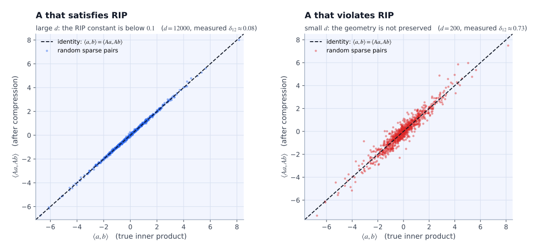
| *Figure 3.1 — The same experiment on two Gaussian matrices. Left: a wide matrix, whose restricted isometry constant is below $0.1$, maps sparse vectors to vectors with almost exactly the same inner products. Right: a narrow matrix, which violates RIP, scrambles them. The band is exactly the RIP guarantee $ | \langle Aa,Ab\rangle-\langle a,b\rangle | \le\delta|a||b|$.* |
3.5.3 Exact recovery by basis pursuit
The ideal recovery problem is
\[\min_{a\in\mathbb R^N}\|a\|_0 \qquad\text{subject to}\qquad Aa=b,\]which is NP-hard in general. Basis pursuit replaces the nonconvex $\ell_0$ with the convex $\ell_1$:
\[\boxed{ \min_{a\in\mathbb R^N}\|a\|_1 \qquad\text{subject to}\qquad Aa=b. }\]Theorem 10 (exact recovery). Let $A$ satisfy the $(2s,\delta)$-RIP with
\[\delta<\sqrt2-1.\]Then every $s$-sparse $a\in\mathbb R^N$ is the unique solution of basis pursuit with measurements $b=Aa$:
\[a=\arg\min_{z\in\mathbb R^N}\bigl\{\|z\|_1 : Az=b\bigr\}.\]This is the classical noiseless recovery theorem of Candès, and the constant $\sqrt2-1\approx 0.4142$ is the standard threshold (Candès 2008; Candès–Tao 2005).
Proof architecture. We give the first step in full, because it is the step that is usually botched, and then state precisely what remains.
| Step 1 (the cone constraint). Let $z$ be any feasible point, $Az=Aa$, and put $h=z-a$; then $Ah=0$. Let $S=\operatorname{supp}(a)$, $ | S | \le s$. If $z$ is a minimizer then $|z|1\le|a|_1$, i.e. $|a+h|_1\le|a|_1$. Splitting $h=h_S+h{S^c}$ and using $a=a_S$, |
By the triangle inequality $|a_S+h_S|_1\ge|a_S|_1-|h_S|_1$, so
\[\boxed{\ \|h_{S^c}\|_1\ \le\ \|h_S\|_1.\ }\]This is the cone constraint: the error made off the true support is bounded by the error made on it. Intuitively, $\ell_1$ recovery fails only if the measurement cannot distinguish “the signal moved slightly” from “the signal moved off the support”, and the cone constraint says the second is always the more expensive option.
Step 2 (the RIP closes the gap). The remaining argument is the content of Candès’ theorem: combine the cone constraint with the RIP, applied to the sparse difference vectors that arise when one decomposes $S^c$ into blocks, to force
\[h_S=0 \quad\text{and}\quad h_{S^c}=0.\]The RIP enters by bounding how much of $h$ the measurement $Ah=0$ can hide; the constant $\sqrt2-1$ is exactly the point at which the resulting geometric comparison flips sign. Two remarks for the reader:
- The proof must be carried out consistently. A common (invalid) version of this argument mixes the $\ell_1$ cone constraint with $\ell_2$ bounds coming from RIP without an intervening $\sqrt{s}$ factor, and then concludes something too strong. When you see a proof of exact recovery, check that the $\ell_1 \to \ell_2$ conversions are explicit.
- Injectivity alone (Prop. 8, i.e. $\delta<1$) is not enough for basis-pursuit recovery. Uniqueness of the sparse solution and optimality of the $\ell_1$ solution are different statements, and the second is what requires $\delta_{2s}<\sqrt2-1$.
Step 3. With $h=0$ we get $z=a$, and $a$ is therefore the unique minimizer. $\qquad\blacksquare$
A note on what RIP does not buy. RIP with $\delta<1$ gives injectivity, i.e. if you already know the code is $s$-sparse and you could solve a nonconvex problem, you would find it. It does not by itself give an algorithm. The $\ell_1$ relaxation is what makes the problem tractable, and the sharp constant $\sqrt2-1$ is what certifies that the relaxation has no slack. This distinction — “the code exists and is unique” versus “the code can be found by a convex program” — is exactly the gap that Part 2 has to bridge in practice, because in a real SAE the dictionary is unknown and the encoder is nonlinear.
3.6 Worked numbers: how many measurements do we need?
Suppose
\[N=10^{6}, \qquad s=20, \qquad \delta=0.1, \qquad \eta=0.01.\]The RIP sample complexity is
\[d\ \gtrsim\ C\,\delta^{-2}\left(s\log\frac Ns+\log\frac1\eta\right).\]Compute:
\[s\log\frac Ns = 20\log\!\left(\frac{10^6}{20}\right) = 20\log(50{,}000) \approx 20\times 10.82 \approx 216.4,\] \[\log\frac1\eta=\log 100\approx 4.61.\]So
\[d\ \gtrsim\ C\cdot 100\cdot(216.4+4.61) \;\approx\; C\cdot 2.21\times10^{4}.\]The exact constant $C$ depends on the proof and the ensemble, but the scaling is the point: the required measurement dimension grows like $s\log(N/s)$, not like $N$. Measuring a signal with $10^6$ unknown coordinates needs only a few tens of thousands of measurements — if the signal is $20$-sparse.
Why this matters for interpretability. A residual stream of width $d=2304$ is not wide enough to satisfy the RIP bound for $N=16{,}384$ features and large $s$ under this crude estimate. That is not a contradiction: the RIP is a worst-case guarantee for random dictionaries over all sparse vectors, whereas a learned SAE dictionary is optimized for the actual activation distribution, which is far from worst case. Part 2 is about how much of the worst-case theory survives when the dictionary is learned rather than random.
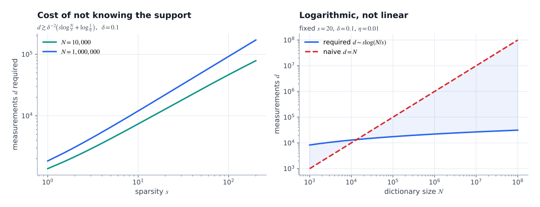
Figure 3.2 — Left: the number of measurements needed grows like $s\log(N/s)$, and is far larger for a bigger dictionary. Right: for fixed sparsity, growing the dictionary from $10^3$ to $10^8$ features costs only a few extra measurements, whereas the naive requirement $d=N$ explodes. This logarithmic scaling is the entire reason a 2304-dimensional residual stream can host a 16,384-feature dictionary.
3.7 The chain so far
\[\boxed{ \text{high-dimensional geometry} \;\longrightarrow\; \text{near-orthogonal packings of size } e^{dt^2/2} \;\longrightarrow\; \text{sparse codes survive compression} \;\longrightarrow\; \text{RIP} \;\longrightarrow\; \text{stable geometry + exact } \ell_1 \text{ recovery}. }\]What Part 1 has established.
- $p_d(t)\le e^{-dt^2/2}$ for all $t\in[0,1]$: in high dimension, a random direction is exponentially far from any fixed direction.
- There exist $\Omega(e^{dt^2/2})$ unit vectors with pairwise inner products at most $t$ — exponentially many “slots” in a $d$-dimensional space.
- A generic linear map $A\in\mathbb R^{d\times N}$ is injective on $\Sigma_s$ iff $d\ge 2s$ (sharp; governed by $\operatorname{spark}(A)=d+1$).
- A Gaussian matrix satisfies $(k,\delta)$-RIP once $d\gtrsim\delta^{-2}(k\log(N/k)+\log(1/\eta))$.
- RIP implies injectivity, and implies inner products are preserved to within $\delta|a||b|$ on sparse vectors — with an explicit coefficient readout $a_i\approx\langle Aa,Ae_i\rangle$.
- Basis pursuit recovers every $s$-sparse vector exactly once $\delta_{2s}<\sqrt2-1$.
What Part 1 has not established. Everything above assumed a random measurement matrix and a known dictionary. In a real model we observe $x\in\mathbb R^d$ and must learn the dictionary and the code at the same time. That is the reversal we make in Part 2.
4. Part 1 Takeaways
- A neural activation is a vector in the residual stream, dimension $d$ fixed by architecture. It is an additive accumulator: every concept the model tracks contributes a direction.
- The bottleneck is real: a model with $d=2304$ must represent far more than $2304$ features. Orthogonality alone cannot solve it.
- Geometry solves the space problem: $\mathbb R^d$ contains exponentially many nearly-orthogonal directions, so “number of features” is not bounded by $d$.
- Sparsity solves the identifiability problem: because only $s$ features are active at a time, a $d$-dimensional measurement can pin them down. The cost is $d = O(s\log(N/s))$, not $O(N)$.
- RIP is the certificate: it converts “sparse codes are recoverable” into a checkable matrix property, and it delivers both geometric stability and exact $\ell_1$ recovery.
- The gap to close: compressed sensing assumes the dictionary is known and random. Interpretability requires the dictionary to be unknown and learned from the model’s own activations. Part 2.
References for Part 1
- E. J. Candès and T. Tao. Decoding by linear programming. IEEE Transactions on Information Theory, 51(12):4203–4215, 2005.
- E. J. Candès, J. Romberg, and T. Tao. Robust uncertainty principles: exact signal reconstruction from highly incomplete frequency information. IEEE Transactions on Information Theory, 52(2):489–509, 2006.
- E. J. Candès. The restricted isometry property and its implications for compressed sensing. Comptes Rendus Mathématique, 346(9–10):589–592, 2008. Exact-recovery threshold: $\delta_{2s}<\sqrt2-1$.
- E. J. Candès, Y. Eldar, D. Mixon, and S. Vempala. An Introduction to Compressed Sensing. Foundations and Trends in Signal Processing, 6(1–4):1–142, 2011.
- R. G. Baraniuk, M. A. Davenport, R. A. DeVore, and M. B. Wakin. A simple proof of the restricted isometry property for random matrices. Constructive Approximation, 28(3):253–263, 2008.
- R. Vershynin. High-Dimensional Probability: An Introduction with Applications in Data Science. Cambridge University Press, 2018. Spherical cap bounds, concentration on the sphere, RIP for sub-Gaussian matrices.
- J. Matoušek. Lectures on Discrete Geometry. Springer, 2002. Background on spherical caps, coverings and packings.
- S. Boyd. Combinatorial Optimization. Cambridge University Press, 2004. Linear programming duality, basis pursuit, $\ell_1$ vs. $\ell_0$.
- R. Tibshirani. Regression shrinkage and selection via the Lasso. Journal of the Royal Statistical Society B, 58(1):267–288, 1996.
Full series bibliography, including the interpretability references used in Parts 2 and 3, appears at the end of Part 3.
Next: Part 2 — Sparse Autoencoders and Superposition. We reverse the compressed-sensing problem: from an observed activation, learn the overcomplete dictionary and the sparse code simultaneously, and ask what the resulting decomposition does and does not prove.
How to cite this article
BibTeX.
@misc{kumar2026geometry1,
  author       = {Kumar, Ajeet},
  title        = {Geometry of Neural Activations, Part 1: High-Dimensional Geometry and Compressed Sensing},
  year         = {2026},
  orcid        = {\url{https://orcid.org/0009-0001-6494-4217}},
  howpublished = {\url{https://ajeetkbhardwaj.github.io/posts/2026/10/geometry-of-neural-activation-part-1/}},
  note         = {Part 1 of Geometry of Neural Activations}
}

© 2026 Ajeet Kumar. This work is licensed under a Creative Commons Attribution 4.0 International License. Credit must be given to the creator.
Comments