Geometry of Neural Activations, Part 2: Sparse Autoencoders and Superposition
Published:
Part 2 of 3. Part 1 established the geometry: in $\mathbb R^d$ there is exponentially much room for directions, and sparsity is what makes a compressed code recoverable. But Part 1 assumed a known, random dictionary. In a real model we observe $x\in\mathbb R^d$ and must learn the dictionary and the code simultaneously. This part is about that reversal, the tool it produces (the sparse autoencoder), and the mathematical picture that tool reveals (superposition).
Table of Contents
- From Compressed Sensing to Dictionary Learning
- 5.1 The reversed problem
- 5.2 The SAE as a dictionary learner
- 5.3 Why there is no canonical dictionary
- 5.4 The alternating scheme
- SAE Architecture and Objective
- 6.1 The ReLU SAE
- 6.2 The objective
- 6.3 Why the decoder must be normalized: the gauge freedom
- 6.4 Why the encoder must be nonlinear
- 6.5 Relation to Lasso, basis pursuit, and sparse coding
- 6.6 Why the code should be nonneg
- SAE Variants
- 7.1 ReLU with an $\ell_1$ penalty
- 7.2 TopK SAE
- 7.3 JumpReLU SAE
- 7.4 Matryoshka SAE
- 7.5 Gated SAEs, and a comparison
- Training and Evaluation
- 8.1 Collecting activations
- 8.2 The empirical objective
- 8.3 The sparsity–fidelity trade-off
- 8.4 Evaluation metrics
- 8.5 Choosing between SAEs
- 8.6 Practical notes
- Interpreting Features
- 9.1 Evidence
- 9.2 Automatic labelling
- 9.3 Simulation, detection, fuzzing
- 9.4 A label is a hypothesis
- Superposition: A Mathematical Model
- 10.1 The regime
- 10.2 What superposition pays: interference
- 10.3 What the Part 1 picture gives, and what it does not
- 10.4 Toy models: importance, frequency, and the frontier
- 10.5 Worked example: Gemma 2 2B
- 10.6 What SAEs establish — and what they do not
- Part 2 Takeaways References for Part 2
5. From Compressed Sensing to Dictionary Learning
5.1 The reversed problem
In classical compressed sensing (Part 1, Chapter 3) the measurement matrix $A\in\mathbb R^{d\times N}$ is known, we observe $b=Aa$, and the task is to recover the sparse vector $a\in\mathbb R^N$.
In mechanistic interpretability the situation is inverted. We observe the activation
\[x\in\mathbb R^{d},\]and we hypothesize that it was produced by a sparse combination of latent features living in a much higher-dimensional space $\mathbb R^N$:
\[x\;\approx\;\sum_{i=1}^{N} f_i(x)\,w_i, \qquad f(x)\in\mathbb R^N_{\ge 0}, \qquad \|f(x)\|_0\ll N, \qquad w_i\in\mathbb R^d,\ \|w_i\|_2=1.\]The unknowns are now both halves of the equation:
| Compressed sensing | Interpretability | |
|---|---|---|
| what is observed | $b=Aa\in\mathbb R^d$ | $x\in\mathbb R^d$ |
| dictionary | known, random | unknown, learned |
| code | to be recovered | unknown, learned |
| model of data | none needed | the model’s activations |
So the task is sparse dictionary learning: learn an overcomplete dictionary $W_{\mathrm{dec}}\in\mathbb R^{d\times N}$ and a sparse code for every input, simultaneously, from data alone.
5.2 The SAE as a dictionary learner
A sparse autoencoder is the standard implementation of this reversal. It has two halves:
\[f_{\mathrm{enc}}:\mathbb R^d\to\mathbb R^N, \qquad g_{\mathrm{dec}}:\mathbb R^N\to\mathbb R^d,\]trained so that
\[x\approx g_{\mathrm{dec}}\bigl(f_{\mathrm{enc}}(x)\bigr) \qquad\text{with}\qquad f_{\mathrm{enc}}(x)\ \text{sparse}.\]Two design decisions carry all the weight:
- The decoder is linear. $g_{\mathrm{dec}}(a)=W_{\mathrm{dec}}a+b_{\mathrm{dec}}$. This makes the decoder literally a dictionary and the reconstruction a linear combination of dictionary atoms. It is what allows us to talk about “feature directions” at all: $w_i=W_{\mathrm{dec}}e_i$ is a direction in activation space that the model can be said to “contain”.
- The encoder is nonlinear and thresholding. $f_{\mathrm{enc}}$ decides which atoms are switched on. Without a nonlinearity there is no notion of a feature being “present” or “absent” (§6.4).
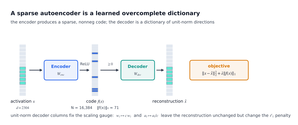
Figure 5.1 — The two halves of an SAE. The encoder maps an activation to a sparse nonneg code; the decoder is a linear dictionary of unit-norm directions; the reconstruction is a linear combination of the active atoms.
5.3 Why there is no canonical dictionary
Dictionary learning is famously non-identifiable. If a dictionary $W$ explains the data, then so do many others: permuting the columns, rescaling columns and their codes in compensating ways, or replacing a group of near-dependent atoms by a different group. Without additional structure, the data does not determine the dictionary.
For SAEs the ambiguity is made worse by two facts:
- The data is a distribution, not a matrix. We do not have “the” code for each activation; we have a cloud of activations and are free to choose codes.
- The dictionary is overcomplete and the model is nonlinear, so the “reconstruction” is a soft constraint, and many dictionaries achieve similar reconstruction quality with different sparsity.
Consequence for interpretation. When we say “feature $i$ means golden gate bridge”, we mean: this particular learned dictionary contains an atom whose activation pattern and causal effect resemble that concept. A different dictionary — different seed, width, or sparsity level — will not contain that atom, and will contain different atoms. This is not a bug in the method; it is a property of the problem. We return to it in Part 3, where it becomes one of the main limitations of the whole enterprise.
Why it still works. In practice, the learned dictionary is far from arbitrary: it is the one that makes the activations both sparse and reconstructible. Across many random seeds and widths, the same concepts recur — not the same atoms, but the same content. The interesting object is therefore not “the dictionary” but “the set of concepts the activation distribution admits a sparse description over”.
5.4 The alternating scheme
The standard training scheme is a two-step alternation (this is the MOD / alternating-minimization scheme of dictionary learning, made practical by the encoder):
- Code step — with $W_{\mathrm{dec}}$ fixed, choose $f(x)$ to make the reconstruction good and the code sparse.
- Dictionary step — with the codes fixed, update $W_{\mathrm{dec}}$ to minimise the reconstruction error.
The nonconvexity of the joint problem is handled by the alternation: each step is convex in its own block, and the usual practice is to add an $\ell_1$ penalty (or a hard sparsity constraint) to the code step so that the code is well-posed.
The encoder $f_{\mathrm{enc}}$ is a parametric surrogate for the code step: instead of solving an optimisation problem for each input, a network is trained to output the solution directly. That is the only real difference between a “dictionary learning” implementation and an “SAE” implementation — and it is why SAEs can be trained on billions of activations.
6. SAE Architecture and Objective
6.1 The ReLU SAE
The standard architecture (Gao et al. 2024) is
\[f(x) = \operatorname{ReLU}\!\left( W_{\mathrm{enc}}\,(x-b_{\mathrm{pre}})+b_{\mathrm{enc}} \right), \qquad \hat x = W_{\mathrm{dec}}\,f(x)+b_{\mathrm{pre}}.\]The pre-activation bias $b_{\mathrm{pre}}$ is subtracted before encoding and added back after decoding, so the SAE is (approximately) an identity map on the mean activation. The reconstruction is therefore
\[\hat x = b_{\mathrm{pre}}+\sum_{i=1}^{N}f_i(x)\,w_i, \qquad w_i=W_{\mathrm{dec}}e_i,\qquad \|w_i\|_2=1.\]Note the shape of this: a nonneg sparse combination of unit-norm directions, plus a constant. This is the same form as the superposition hypothesis from §1.2, with $a_i=f_i(x)$.
6.2 The objective
\[\boxed{ \mathcal L = \mathbb E_x\left[ \|x-\hat x\|_2^2 + \lambda\,\|f(x)\|_1 \right]. }\]The first term rewards faithful reconstruction; the second penalises total activation mass. Because the code is nonneg, $|f(x)|_1=\sum_i f_i(x)$ is exactly the “total feature activity” on that input, and $\lambda$ sets the exchange rate between reconstruction error and feature mass.
The two terms pull in opposite directions, and their relative size determines the operating point of the SAE (§8.3). Note that this objective is a population objective; in practice one uses the empirical average over a large dataset of recorded activations (§8.2).
6.3 Why the decoder must be normalized: the gauge freedom
This is the single most important structural detail of the architecture, and it is easy to get wrong.
Let $w_i$ be the $i$-th decoder column and $f_i$ the corresponding encoder activation. Their contribution to the reconstruction is the product $f_iw_i$. Now rescale:
\[w_i\longmapsto c\,w_i, \qquad f_i\longmapsto c^{-1}f_i, \qquad c>0.\]Then
\[f_iw_i\;\longmapsto\;(c^{-1}f_i)(cw_i)=f_iw_i,\]so the reconstruction is unchanged, and the reconstruction loss is unchanged. But the sparsity penalty is not:
\[\lambda|f_i|\;\longmapsto\;\lambda c^{-1}|f_i|.\]For $c>1$ the penalty decreases. Therefore, without a constraint on the decoder scale, the optimiser can drive the total objective down by inflating decoder columns and shrinking the corresponding activations, without changing the represented information at all.
Precise statement. The objective
\[\mathbb E_x\bigl[\|x-\hat x\|_2^2+\lambda\|f(x)\|_1\bigr]\]has a scaling gauge freedom: the map $(w_i,f_i)\mapsto(cw_i,c^{-1}f_i)$ leaves the first term invariant and decreases the second for $c>1$. The standard gauge fix is to impose unit-norm decoder columns:
\[\boxed{\ \|W_{\mathrm{dec}}e_i\|_2=1\quad\text{for every }i.\ }\]With this constraint, $f_i(x)$ acquires a precise geometric meaning: it is the length of the component of the activation along the unit direction $w_i$, contributed by feature $i$. It also fixes the scale of every feature, which is what makes features comparable across dictionaries and across layers.
A correction worth stating explicitly. This has nothing to do with Lasso being “scale-invariant”. Ordinary Lasso on a fixed dictionary is not scale-invariant, and neither is the SAE objective. The point is narrower: the SAE objective has a gauge freedom, and unit-norm decoder columns remove it.
6.4 Why the encoder must be nonlinear
Suppose the encoder and decoder were both linear and bias-free:
\[f_{\mathrm{enc}}(x)=Ux, \qquad g_{\mathrm{dec}}(a)=Va.\]Then the composite map is linear:
\[g_{\mathrm{dec}}\bigl(f_{\mathrm{enc}}(x)\bigr)=VUx.\]A linear autoencoder of rank $r$ can only learn an $r$-dimensional linear subspace of $\mathbb R^d$ — essentially principal component analysis. It cannot produce an overcomplete sparse code, because “which coordinates are active” is not a property a linear map can express: any linear map is surjective onto its image and has a trivial kernel structure. Sparsity requires a selection, and selection requires a nonlinearity.
The ReLU is the simplest useful nonlinearity, and it performs exactly the selection we want:
\[f_i(x)=\operatorname{ReLU}\!\left(\langle W_{\mathrm{enc},i},\,x-b_{\mathrm{pre}}\rangle+b_i\right).\]Feature $i$ is active exactly when its pre-activation is positive. The set of active features is therefore a region of activation space cut out by hyperplanes — a piecewise-linear selection, and a hard one, which is what makes the code sparse and conditionally active.
6.5 Relation to Lasso, basis pursuit, and sparse coding
Compare three objectives on a fixed dictionary $W\in\mathbb R^{d\times N}$:
Basis pursuit (Part 1, §3.5.3)
\[\min_a\|a\|_1\quad\text{s.t.}\quad Wa=b.\]Lasso
\[\min_a\frac12\|b-Wa\|_2^2+\lambda\|a\|_1.\]SAE (with $W$ learned)
\[\min_{W_{\mathrm{enc}},W_{\mathrm{dec}}} \mathbb E_x\left[\frac12\|x-W_{\mathrm{dec}}f_{\mathrm{enc}}(x)\|_2^2+\lambda\|f_{\mathrm{enc}}(x)\|_1\right].\]The SAE has the same shape as Lasso — squared error plus $\ell_1$ — but three things differ:
- The dictionary is learned, not fixed. This is the crucial difference: the object being estimated is the set of feature directions, not just the code.
- The code is produced parametrically, by the encoder, rather than by solving an optimisation problem per input.
- The code is constrained nonneg, which removes sign ambiguity in the atoms and makes “feature present” a single-sided notion.
So an SAE is closer to sparse coding / dictionary learning than to Lasso. The Lasso is the special case where the dictionary is given and only the code is estimated.
6.6 Why the code should be nonneg
Requiring $f_i(x)\ge0$ is not cosmetic:
- It fixes the sign of every atom. Without it, $w_i$ and $-w_i$ are equally good, and the sign of a feature becomes an artefact of initialisation.
- It makes a feature’s presence interpretable as a magnitude. A feature that is “on” contributes a fixed direction with a positive weight, and a feature that is “off” contributes nothing.
- It matches the ReLU encoder, which produces nonneg pre-activations by construction.
The cost is a modelling restriction: a genuinely bipolar concept (e.g. “not X” versus “X”) must be represented by two atoms, one for each sign. In practice this is a good trade.
7. SAE Variants
All variants share the same skeleton — a nonlinear encoder producing a sparse code, a linear decoder of unit-norm atoms — and differ in how sparsity is enforced. That single axis determines most of their practical behaviour.
7.1 ReLU with an $\ell_1$ penalty
\[f(x)=\operatorname{ReLU}\!\left(W_{\mathrm{enc}}(x-b_{\mathrm{pre}})+b_{\mathrm{enc}}\right), \qquad \mathcal L=\mathbb E_x\left[\|x-\hat x\|_2^2+\lambda\|f(x)\|_1\right].\]Sparsity is encouraged by a penalty. Consequence: the number of active features varies from input to input, and $\lambda$ is a soft knob. Large $\lambda$ → sparser codes, worse reconstruction. Small $\lambda$ → dense codes, better reconstruction. There is no guarantee that a given feature is ever switched on; the $\ell_1$ penalty can simply zero out an uninformative atom.
7.2 TopK SAE
Let $z=W_{\mathrm{enc}}(x-b_{\mathrm{pre}})+b_{\mathrm{enc}}$. Define
\[f(x)=\operatorname{TopK}\!\left(\operatorname{ReLU}(z)\right),\]where $\operatorname{TopK}$ keeps the $k$ largest positive coordinates and zeroes the rest. The objective is then pure reconstruction:
\[\mathcal L=\mathbb E_x\left[\|x-\hat x\|_2^2\right].\]Key distinction. In a ReLU+$\ell_1$ SAE, sparsity is a penalty and the code is only approximately sparse. In a TopK SAE, sparsity is architectural: $|f(x)|_0\le k$ holds for every input, by construction, and $k$ is a direct, interpretable control. There is no $\lambda$ to tune and no trade-off knob inside the objective — the trade-off is between different values of $k$.
TopK also has a failure mode worth naming: because the selection is hard, a feature that is almost selected can be dropped entirely, and a small change in $x$ can swap which features are on. This produces “chattering” in downstream analyses (a feature flickering on and off across near-identical prompts) unless the code is post-processed.
7.3 JumpReLU SAE
JumpReLU gives each feature its own learned threshold. With
\[z_i=\langle W_{\mathrm{enc},i},x-b_{\mathrm{pre}}\rangle+b_i,\]define
\[f_i(x)=z_i\,\mathbf 1\{z_i\ge\theta_i\},\]where $\theta_i$ is a learned parameter. The feature is off below its threshold and on (with value $z_i$) above it.
The objective penalises the expected number of active features:
\[\mathcal L = \mathbb E_x\left[\|x-\hat x\|_2^2+\lambda\|f(x)\|_0\right], \qquad \|f(x)\|_0=\#\{i:f_i(x)>0\}.\]Two notes:
- The $\ell_0$ term is non-differentiable. Practical implementations use a surrogate gradient or a straight-through estimator around the thresholding operation.
- JumpReLU is a “budget” formulation: choose a target $L_0$, and the model learns thresholds that hit it while minimising reconstruction error. It also yields a reconstruction of the whole activation that is exact for the atoms that fire — the “jump” is a hard threshold, so the decoder output is a sum of selected atoms with no shrinkage.
7.4 Matryoshka SAE
A Matryoshka SAE requires that every prefix of the dictionary be a usable dictionary. Let
\[M=\{m_1<m_2<\dots<m_J=N\}\]be a set of prefix sizes, and define the prefix reconstruction
\[\hat x^{(m)}=b_{\mathrm{pre}}+\sum_{i=1}^{m}f_i(x)\,w_i.\]The nested objective is
\[\mathcal L = \sum_{m\in M}\mathbb E_x\left[\|x-\hat x^{(m)}\|_2^2\right].\]So the first $m_1$ features must reconstruct $x$ on their own, the first $m_2$ features must reconstruct $x$, and so on. This encourages a hierarchy: early features capture broad or high-frequency structure, later features refine it, and every prefix remains a usable partial dictionary. The practical payoff is that one trained SAE gives you a family of SAEs at different widths, and the prefixes are ordered by importance.
7.5 Gated SAEs, and a comparison
Gated SAEs add a learned gate that multiplicatively modulates the encoder output, so the sparsity penalty applies to the gated code while the reconstruction uses the ungated one. This decouples “which features are allowed to fire” from “how strongly they fire”, and gives better reconstruction at a given $L_0$.
| Variant | Sparsity enforced by | Knob | Code shape |
|---|---|---|---|
| ReLU +$\ell_1$ | penalty | $\lambda$ | variable$\ell_0$, soft |
| TopK | architecture | $k$ | exactly$k$ (hard) |
| JumpReLU | learned thresholds + expected$\ell_0$ | budget | thresholded, with per-feature$\theta_i$ |
| Matryoshka | prefix reconstruction | prefix set | nested, ordered by importance |
| Gated | gate + penalty | $\lambda$, budget | gated magnitude |
8. Training and Evaluation
8.1 Collecting activations
To train an SAE on a language model:
- Choose an activation site — e.g. the residual stream after layer $\ell$.
- Run a large text corpus through the model.
- Record the activation vector $x\in\mathbb R^d$ at every token position.
- Assemble a dataset $\mathcal D={x_1,\dots,x_n}\subseteq\mathbb R^d$.
Typical SAE training sets contain $10^9$–$10^{10}$ activation vectors. Two practical decisions matter:
- Which tokens. Using every token position over-represents boilerplate. Many pipelines subsample, or restrict to positions where the model is doing something interesting.
- Which layer. Early layers are more lexical, later layers more semantic; the same activation site supports very different features.
8.2 The empirical objective
For a dataset of $n$ recorded activations, the empirical ReLU+$\ell_1$ objective is
\[\boxed{ \mathcal L_{\mathrm{emp}} = \frac1n\sum_{j=1}^{n} \left( \|x_j-\hat x_j\|_2^2 + \lambda\|f(x_j)\|_1 \right). }\]The design choices are: the activation site; the dictionary width $N$; the sparsity knob ($\lambda$, or TopK’s $k$); the architecture; and the training distribution.
8.3 The sparsity–fidelity trade-off
The central empirical fact about SAEs is a trade-off: you can have a sparse code or an accurate reconstruction, and every point in between is a choice.
The figure below is a measured trade-off curve, produced by the same alternating-minimization dictionary learner used elsewhere in this series, run on synthetic superposition data ($d=48$ dimensions, $N=256$ atoms, ground-truth sparsity $s=6$), with the code-sparsity budget $k$ swept from $2$ to $45$:
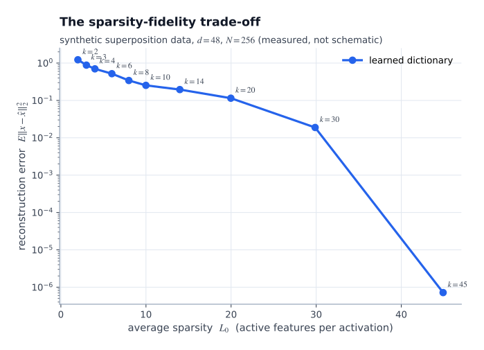
Figure 8.1 — Sparsity versus reconstruction error, measured (not schematic) on a synthetic dictionary-learning problem. Each point is a fully trained dictionary at the indicated sparsity budget $k$. Reading it: at $L_0\approx 10$ the model still explains only part of the variance; by $L_0\approx 45$ — well above the true sparsity of $6$ — the reconstruction is essentially exact. The curve is monotone and steep, which is why the choice of operating point matters more than the choice of algorithm.
Two qualitative features generalize to real SAEs:
- The curve is monotone: more active features, less reconstruction error.
- The curve has a knee: below some $L_0$, adding features buys a lot of reconstruction; above it, features are added that barely help. Choosing the operating point is choosing where to sit relative to the knee.
The synthetic experiment also shows why the learned dictionary matters: with a fixed budget $k$, the alternation recovers a dictionary that reconstructs well and keeps the code at $k$ active atoms. The sparsity is not a mask applied to a dense representation; it is what shapes the dictionary.
8.4 Evaluation metrics
Average sparsity
\[\boxed{ L_0=\mathbb E_x\left[\#\{i:f_i(x)>0\}\right]. }\]How many features are active on a typical token. This is the quantity that the sparsity knob controls directly.
Fraction of variance explained
Let $\mu=\mathbb E_x[x]$. Define
\[\boxed{ \mathrm{FVE} = 1-\frac{\mathbb E_x\|x-\hat x\|_2^2}{\mathbb E_x\|x-\mu\|_2^2}. }\]The fraction of variance in the activation distribution explained by the reconstruction. $\mathrm{FVE}=1$ is a perfect reconstruction; $\mathrm{FVE}=0$ means the SAE explains no more than predicting the mean. (Note that this metric ignores the sparsity of the code entirely, so it must be read together with $L_0$.)
Downstream loss increase
Replace the original activation $x$ by its reconstruction $\hat x$ inside the model, and measure the increase in next-token prediction loss:
\[\boxed{ \Delta\mathrm{CE} = \mathbb E_{\text{text}}\left[\mathrm{CE}_{\mathrm{SAE}}-\mathrm{CE}_{\mathrm{clean}}\right]. }\]with $\mathrm{CE}$ in nats. This is the only causal metric of the three: it tests whether the SAE reconstruction preserves the model’s actual computational behaviour, rather than just approximating it in $\ell_2$.
8.5 Choosing between SAEs
The right way to compare two SAEs is a curve, not a point. Train several SAEs with different $\lambda$ (or different $k$), evaluate each on held-out text, and plot
\[\text{downstream loss increase}\quad\text{against}\quad L_0.\]A better SAE is the one lower down: for the same tolerated loss increase, it uses fewer active features. Equivalently, for the same $L_0$, it costs less downstream loss.
The usual protocol fixes a loss budget — for example $0.1$ nats — and picks the architecture/hyperparameter that reaches the desired sparsity within that budget. In the lecture this series is based on, the illustrative comparison at a $0.1$-nat budget was roughly $L_0\approx 43$ for a TopK SAE versus $L_0\approx 410$ for a ReLU+$\ell_1$ SAE. These are empirical numbers from one setup, not constants: they depend on the model, the layer, the dataset, the dictionary width, and the training recipe, and they should always be re-measured before being quoted.
8.6 Practical notes
Training an SAE is easy to do badly. The recurring failure modes:
- Dead features. An atom that never fires receives no gradient and stays dead. Fixes: reinitialise dead atoms from high-error residuals, and/or resample dead atoms from a “revived” pool.
- Auxiliary loss blow-up. The reconstruction term and the auxiliary (sparsity) loss live on different scales, so a naive sum is badly balanced. Common practice: normalise the reconstruction loss (e.g. divide by $|x-\hat x|_2^2$) and tune the auxiliary coefficient on a log-scale.
- Unstable early training. Large learning rates on the decoder cause the dictionary to thrash. Standard practice: lower learning rates for the decoder, and normalise decoder columns after each step.
- Batch-size effects. Larger batches (more distinct activations per step) produce better-conditioned updates; the standard advice is “as many activations per batch as memory allows”.
9. Interpreting Features
An SAE gives you a dictionary. To say anything interesting about it, you have to find out what the atoms respond to.
9.1 Evidence
For a feature $i$, the primary evidence is the set of texts on which it activates:
- the texts where $f_i(x)$ is largest;
- examples with lower but nonzero activation;
- the tokens on which the feature activates;
- the output tokens promoted by the feature direction $w_i$.
The last item uses the fact that the decoder direction can be compared with the model’s unembedding matrix. If the unembedding vector $u_t$ of token $t$ has a large inner product with $w_i$,
\[\langle w_i,u_t\rangle>0,\]then pushing the residual stream along $w_i$ increases the logit of token $t$. This is the bridge from “the feature fires on Golden” to “the feature would make the model say Golden”.
9.2 Automatic labelling
The standard pipeline:
- Find texts and token positions where feature $i$ activates strongly.
- Give those examples to a language model.
- Ask the model to write a short description of the common pattern.
- Treat the description as a hypothesis about the feature.
For example, a feature may activate strongly on occurrences of “Golden” in names, on gold as a material or colour, on bridge-related language, or on San Francisco Bay Area references.
9.3 Simulation, detection, fuzzing
To test a label, three increasingly direct methods are used.
Simulation. Give a second model only the feature’s description and ask it to predict the feature’s activation on new texts. Compare predicted and true activations, e.g. by correlation. This tests whether the description encodes the pattern.
Detection. Give the second model a set of texts and ask it to pick out which ones activate the feature. Compare with ground truth. This tests whether the description identifies the pattern.
Fuzzing. Give the model positive and negative examples and ask it to distinguish activating from non-activating contexts. This tests whether the description is usable as a discriminator, and is the closest of the three to the way the feature is actually used by the model.
All three measure the same thing in different guises: whether the natural-language description captures the feature’s activation pattern.
9.4 A label is a hypothesis
None of these methods is a proof, and the difference matters. A label is a hypothesis about $f_i$; simulation, detection and fuzzing are its tests; and activation steering (Part 3, Chapter 12) is a causal test of the hypothesis. The natural-language label is a compression of the activation pattern, and compression loses information: two features with different patterns can receive the same label, and one feature with a broad pattern can receive a label that is only true of part of its support.
This is why the downstream workflow is: label → test → steer → refine. Each step can fail, and failure is informative.
10. Superposition: A Mathematical Model
We now have the tool. What does it reveal about the geometry of activations?
10.1 The regime
Let
- $d$ be the residual-stream dimension,
- $N$ be the number of latent features,
- $s$ be the number of features active in a typical activation.
The superposition regime is
\[\boxed{ s\;\ll\; d \;\ll\; N. }\]The network stores $N$ feature directions in only $d$ dimensions. Since $N>d$, those directions cannot all be mutually orthogonal in $\mathbb R^d$; they must interfere. Superposition is the hypothesis that networks organise that interference so that it is tolerable: features that are active together are (nearly) non-interfering, and features that are never active together are free to overlap.
10.2 What superposition pays: interference
The right object for measuring interference is the Gram matrix of the learned dictionary:
\[G=W_{\mathrm{dec}}^\top W_{\mathrm{dec}}\in\mathbb R^{N\times N}, \qquad G_{ij}=\langle w_i,w_j\rangle.\]By the unit-norm constraint, $G_{ii}=1$: the diagonal is fixed. The off-diagonal mass is the interference — the part of the representation that is not a clean sum of independent features. And the only interference that matters is the interference between features that are active at the same time:
\[\text{interference that the model actually pays} = \big\langle w_i,w_j\big\rangle \quad\text{for pairs } (i,j) \text{ that co-occur}.\]The figure below makes this concrete. Panel (a) is a designed dictionary: ten orthonormal bases in $\mathbb R^{100}$, where atoms within a group are exactly orthogonal and atoms across groups overlap randomly. This is the geometric content of superposition — organised so that co-active atoms do not interfere. Panel (b) is a dictionary learned by alternating minimization on synthetic data whose ground-truth atoms were themselves random. Panel (c) compares the two.
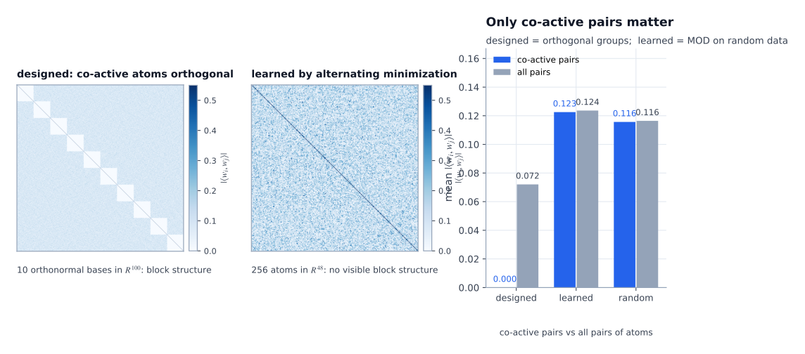
| *Figure 10.1 — Interference geometry. (a) A designed dictionary of ten orthonormal bases in $\mathbb R^{100}$: co-active pairs have $ | \langle w_i,w_j\rangle | =0$ exactly, while all pairs average $0.072$. (b) A dictionary learned by alternating minimization on synthetic data with random ground-truth atoms: no block structure. (c) The summary — mean $ | \langle w_i,w_j\rangle | $ for co-active pairs versus all pairs, for the designed dictionary, the learned dictionary, and the random initialisation.* |
| The measured numbers are instructive, and they include a negative result: the learned dictionary’s co-active pairs average $ | \langle w_i,w_j\rangle | = 0.1225$, against $0.1236$ for all pairs — essentially no separation. But the data in that experiment had random ground-truth atoms, so there was no co-active orthogonality to find. The optimiser faithfully reproduced the structure that was present, and the structure was absent. |
Three conclusions:
- Interference is local, not global. A dictionary need not be orthogonal to be usable; it only needs the active subset to be well-conditioned. This is the sparse-view of Part 1: the RIP-type statements are statements about $\Sigma_s$, not about the whole of $\mathbb R^N$.
- The organisation of interference is a property of the model, not of the optimizer. The learned dictionary inherits whatever geometry the network’s computation imposes on its features. If the model separates two features, an SAE can find them separated; if the model does not, no training procedure will manufacture the separation.
- This is exactly the RIP picture, one level up. Part 1 asked when a random projection preserves the geometry of $s$-sparse vectors. A trained SAE is asking the same question of a learned dictionary, and the answer is: the learned dictionary is optimised to make the active subsets well-conditioned on the actual activation distribution, rather than on all sparse vectors.
10.3 What the Part 1 picture gives, and what it does not
From Part 1 we have: if $A$ satisfies the $(2s,\delta)$-RIP, then for $a,b\in\Sigma_s$,
\[\left|\langle Aa,Ab\rangle-\langle a,b\rangle\right|\le\delta\|a\|\|b\|.\]The natural (and common) move is to read a trained SAE as if it were such an $A$: the code lives in $\mathbb R^N$, the activation is $Ax$ with $x=W_{\mathrm{dec}}^\top(x-b_{\mathrm{pre}})$-ish, and “the SAE is a compressed-sensing decoder that learned its own measurement matrix”.
This reading needs care, and it is worth being precise about which parts transfer:
- What transfers: the qualitative structure. Sparsity plus a well-conditioned active subset gives recoverable, readable features. The $s\ll d\ll N$ regime, the $\log$ scaling of the required width, and the role of the active set are all real.
- What does not transfer: the guarantees. The RIP theorems are worst-case statements about random matrices over all $s$-sparse vectors. A trained SAE’s dictionary is optimised for one specific activation distribution, and nothing about it is uniform over $\Sigma_s$. In particular, a learned dictionary may be perfectly conditioned on the supports that occur in practice and badly conditioned on supports that never occur — which is exactly what we want, and exactly what a worst-case guarantee cannot give.
- What the SAE adds: the nonlinearity. A true compressed-sensing recovery would solve an optimisation problem per input. An SAE amortises that: the encoder is a trained, reusable approximation to the solver. This is a genuine conceptual advance over Part 1 — it is what makes the theory usable at the scale of a language model.
10.4 Toy models: importance, frequency, and the frontier
The cleanest formalisation of superposition is Elhage et al.’s toy models (2022), which are small networks trained from scratch on synthetic datasets with a known number of features. The setup:
- There are $N$ features with importances $I_1,\dots,I_N$ (each feature is a binary or continuous variable with a given variance/importance) and frequencies $f_1,\dots,f_N$ (how often it is active).
- The network has $d$ dimensions and must represent all $N$ features.
- The question is: for which $(I,f,d)$ does the network represent all features, and how does it choose to trade off?
The empirical result is a Pareto frontier rather than a threshold. If features are roughly equally important and equally frequent, the network uses superposition and represents all of them, at the cost of interference. If some features are much more important, the network sacrifices the unimportant ones: it dedicates orthogonal directions to the important features and lets the unimportant ones share (and corrupt) the leftovers.
This gives superposition a quantitative character:
- there is a notion of capacity — the number of features that can be represented, which grows with $d$ but more slowly than $d$ when features are numerous;
- there is a trade-off between how many features are represented and how much interference the represented ones suffer;
- the boundary is not a sharp threshold but a frontier, and the operating point depends on the importance and frequency distributions, not only on $d$ and $N$.
The framework also makes the “importance” concept concrete: a feature that fires rarely but matters a lot (e.g. a safety-relevant concept) behaves very differently from a feature that fires constantly and matters little. This is why sparsity alone is not the whole story — which features are active matters as much as how many.
10.5 Worked example: Gemma 2 2B
For Gemma 2 2B,
\[d=2304.\]A Gemma Scope SAE on the residual stream at layer 20 used
\[N=16{,}384, \qquad L_0\approx 71.\]So on a typical token, roughly $71$ of $16{,}384$ features were active:
\[\frac{71}{16{,}384}\approx 0.43\%.\]And the SAE width was about $7.1\times$ the residual-stream dimension:
\[\frac Nd=\frac{16{,}384}{2304}\approx 7.1.\]This is a concrete superposition regime:
\[L_0\ll d\ll N.\]Two things are worth noticing. First, $L_0\approx71$ is not small compared to $d=2304$: a typical activation has dozens of features on at once, and they are definitely not orthogonal. Second, $N/d\approx7$ is far below what the geometry of Part 1 permits — at $d=2304$ one could pack on the order of $10^{14}$ near-orthogonal directions (§2.5), so a width of $16{,}384$ is using a tiny fraction of the available room. The binding constraint on the number of features is therefore not the geometry of the space; it is the identifiability and interpretability of the learned decomposition, and the compute used to train it.
10.6 What SAEs establish — and what they do not
What an SAE establishes. The activation distribution admits a sparse, overcomplete, often highly interpretable description. Early work (Bricken et al. 2023) found features more monosemantic than individual neurons, including features responding to specific scripts, biological sequences, and encoding formats. Later work (Templeton et al. 2024) found features in Claude 3 Sonnet for things like the Golden Gate Bridge, with clean, nameable semantics.
What an SAE does not establish. That the original network literally computes using those features. The SAE shows that the activations can be described that way; it does not show that the network does it that way. The distinction is the difference between a description of a representation and a mechanism for a computation.
The failure modes, concretely:
- Feature splitting. One concept may be represented by several features; a wider dictionary fragments it further (see Part 3, §17.3).
- Feature absorption. Several related concepts may be merged into one feature.
- Reconstruction–sparsity trade-off. Large $\lambda$ gives sparser but less faithful codes.
- Dictionary non-uniqueness. Many dictionaries reconstruct the same distribution equally well (§5.3).
- Dead features and training instability. Practical SAEs need careful initialisation, normalisation, learning-rate schedules, and resampling.
- Unexplained variance. Even very wide SAEs leave nonzero reconstruction error; the residue is sometimes called the dark matter of SAEs.
11. Part 2 Takeaways
- The problem is inverted. We do not recover a code from a known measurement matrix; we learn the matrix and the code together, from activations alone. This is sparse dictionary learning.
- A ReLU SAE is $x\approx b_{\mathrm{pre}}+\sum_i f_i(x)w_i$ with $f(x)\ge0$, sparse, and $|w_i|_2=1$.
- Unit-norm decoder columns are a gauge fix, not a stylistic choice: without them the objective has a scaling freedom that lets the optimiser shrink the penalty without changing the information.
- The encoder must be nonlinear, because sparsity is a selection and a linear map cannot select; a linear autoencoder is PCA.
- Sparsity can be enforced by a penalty (ReLU+$\ell_1$), architecturally (TopK), by learned thresholds (JumpReLU), or structurally across prefixes (Matryoshka).
- The sparsity–fidelity trade-off is the central empirical fact; the operating point is chosen from a curve, not a number.
- Evaluation must be causal: reconstruction error and FVE are necessary but not sufficient; the downstream loss increase is the metric that tests whether the SAE preserved the computation.
- A label is a hypothesis, tested by simulation, detection and fuzzing, and ultimately by steering.
- Superposition is the regime $s\ll d\ll N$, and its currency is interference — the off-diagonal mass of the dictionary Gram matrix, paid only between co-active features.
- What SAEs show is that the activations admit a sparse, interpretable description — not that the network computes with those features. That distinction is where Part 3 begins.
References for Part 2
- A. Bricken, A. Templeton, J. Batson, B. Chen, A. Jermyn, T. Conerly, et al. Towards monosemanticity: decomposing language models with dictionary learning. Transformer Circuits Thread, 2023.
- H. Cunningham, A. Ewart, L. Riggs, R. Huben, and L. Sharkey. Sparse autoencoders find highly interpretable features in language models. ICLR, 2024. arXiv:2309.08600.
- A. Templeton, T. Conerly, J. Marcus, J. Lindsey, T. Bricken, B. Chen, et al. Scaling monosemanticity: extracting interpretable features from Claude 3 Sonnet. Transformer Circuits Thread, 2024.
- L. Gao, T. Dupré la Tour, H. Tillman, G. Goh, R. Troll, A. Radford, I. Sutskever, J. Leike, and J. Wu. Scaling and evaluating sparse autoencoders. arXiv:2406.04093, 2024.
- S. Rajamanoharan, T. Conerly, A. Jermyn, N. Nanda, J. Leike, and T. Bricken. Jumping ahead: improving reconstruction fidelity with JumpReLU sparse autoencoders. arXiv:2407.14435, 2024.
- B. Bussmann, P. Leask, and N. Nanda. Learning multi-level features with Matryoshka sparse autoencoders. ICML, 2025. arXiv:2503.17547.
- T. Lieberum, S. Rajamanoharan, A. Conmy, L. Smith, N. Nanda, et al. Gemma Scope: open sparse autoencoders everywhere all at once on Gemma 2. arXiv:2408.05147, 2024.
- N. Elhage, T. Hume, C. Olsson, N. Schiefer, T. Henighan, S. Kravec, et al. Toy models of superposition. Transformer Circuits Thread, 2022. arXiv:2209.10652.
- E. J. Mairal, P. Calandrino, and J. Ponce. Online dictionary learning for sparse coding. ECCV, 2010. (MOD, the alternating scheme.)
- A. M. Bruckstein, D. Donoho, and M. Elad. Sparse solutions for underdetermined systems of linear equations. IEEE Transactions on Information Theory, 42(2):407–425, 1996. (Sparse coding / dictionary learning.)
- M. Aharon and M. Elad. Sparse and redundant representation modeling: dictionary learning. (Gated SAE / LASSO dictionary learning.)
- R. Tibshirani. Regression shrinkage and selection via the Lasso. Journal of the Royal Statistical Society B, 58(1):267–288, 1996.
- G. Billis, S. Marks, J. Bricken, et al. Language models can explain neurons in language models. OpenAI, 2023. (Automatic interpretability: simulation, detection, fuzzing.)
- G. Paulo, A. Mallen, C. Juang, and N. Belrose. Automatically interpreting millions of features in large language models. 2024. (Massive-scale auto-labelling.)
- A. Conmy, et al. Scaling up the evaluation of sparse autoencoders. 2023. Introduces the standard evaluation battery: $L_0$, fraction of variance explained, and downstream cross-entropy increase.
The full series bibliography continues in Part 3.
Next: Part 3 — Steering, Linear Structure, and Feature Manifolds. We take a feature and pull on it: intervention, clamping, alignment applications, the linear representation hypothesis, and the nonlinear structure that a sparse linear dictionary cannot capture.
How to cite this article
BibTeX.
@misc{kumar2026geometry2,
  author       = {Kumar, Ajeet},
  title        = {Geometry of Neural Activations, Part 2: Sparse Autoencoders and Superposition},
  year         = {2026},
  orcid        = {\url{https://orcid.org/0009-0001-6494-4217}},
  howpublished = {\url{https://ajeetkbhardwaj.github.io/posts/2026/10/geometry-of-neural-activation-part-2/}},
  note         = {Part 2 of Geometry of Neural Activations}
}

© 2026 Ajeet Kumar. This work is licensed under a Creative Commons Attribution 4.0 International License. Credit must be given to the creator.
Comments