Geometry of Neural Activations, Part 3: Steering, Linear Structure, and Feature Manifolds
Published:
Geometry of Neural Activations — Part 3
Steering, Linear Structure, and Feature Manifolds
Part 3 of 3. Parts 1 and 2 built the geometry and the instrument. This part asks the questions that make the instrument worth having: does a feature cause behaviour, what does the shape of a concept look like in activation space, and what does a sparse linear dictionary fundamentally fail to capture?
Table of Contents
- From Correlation to Intervention
- 12.1 Additive steering
- 12.2 Feature clamping
- 12.3 The two interventions compared
- 12.4 Why clamping can preserve coherence
- Case Study: The Golden Gate Bridge
- 13.1 The experiment
- 13.2 What it established
- 13.3 What it did not
- Applications to Alignment and Safety
- 14.1 Model diffing with SAEs
- 14.2 Emergent misalignment
- 14.3 Refusal, sycophancy, and unsafe code
- 14.4 The dual-use problem
- The Linear Representation Hypothesis
- 15.1 The statement
- 15.2 Word2vec-style structure
- 15.3 Why softmax encourages linear contrasts
- 15.4 The logit lens
- 15.5 Caveats
- Feature Manifolds
- 16.1 Definition
- 16.2 Four examples
- 16.3 Manifold-aware steering
- 16.4 The general recipe
- Limitations of Sparse Autoencoders
- 17.1 Dark matter
- 17.2 No canonical dictionary
- 17.3 Feature splitting and absorption
- 17.4 Hierarchical concepts
- 17.5 Nonlinear structure
- Open Problems and the Research Program
- 18.1 Manifold-aware SAEs
- 18.2 Unsupervised manifold discovery
- 18.3 Better evaluation
- 18.4 The program
- 18.5 Part 3 takeaways
- The Series Bibliography
12. From Correlation to Intervention
Finding that a feature $f_i$ activates on certain texts establishes, at best, a correlation between the feature and a concept. The concept of a feature being causally responsible for behaviour requires an intervention.
12.1 Additive steering
Let $x\in\mathbb R^d$ be a residual-stream activation at a chosen site, and let
\[w_i=W_{\mathrm{dec}}e_i\in\mathbb R^d\]be the decoder direction of SAE feature $i$. The simplest intervention is additive steering:
\[\boxed{ x\;\longleftarrow\;x+\alpha w_i. }\]Here $\alpha\in\mathbb R$ is the steering strength.
- $\alpha>0$ increases the model’s exposure to the direction $w_i$.
- $\alpha<0$ suppresses it.
- $\alpha=0$ leaves the model unchanged.
The modified vector is written back into the residual stream and the forward pass continues normally. Because the intervention happens inside the network, the effect propagates through all subsequent layers — we are not editing the output, we are changing the state.
12.2 Feature clamping
Additive steering has a limitation: the residual stream may already contain a substantial component along $w_i$. Adding $\alpha w_i$ changes the total coefficient, but does not set it. And the natural coefficient varies from token to token, so the same $\alpha$ produces a different effective intervention at different positions.
To set the feature to a chosen value, first remove the existing component along $w_i$, then add the desired amount. Assuming $|w_i|_2=1$, the component of $x$ along $w_i$ is $\langle x,w_i\rangle w_i$, so define
\[\boxed{ x_{\mathrm{clamp}} = x-\langle x,w_i\rangle w_i+c\,w_i = x+\bigl(c-\langle x,w_i\rangle\bigr)w_i. }\]Then, by construction,
\[\langle x_{\mathrm{clamp}},w_i\rangle=c.\]The difference is precise: steering shifts the coefficient by a constant; clamping sets it to a constant.
12.3 The two interventions compared
| Intervention | Formula | Effect on the coefficient |
|---|---|---|
| Additive steering | $x+\alpha w_i$ | $\langle x,w_i\rangle+\alpha$ |
| Clamping | $x-\langle x,w_i\rangle w_i+c\,w_i$ | exactly$c$ |
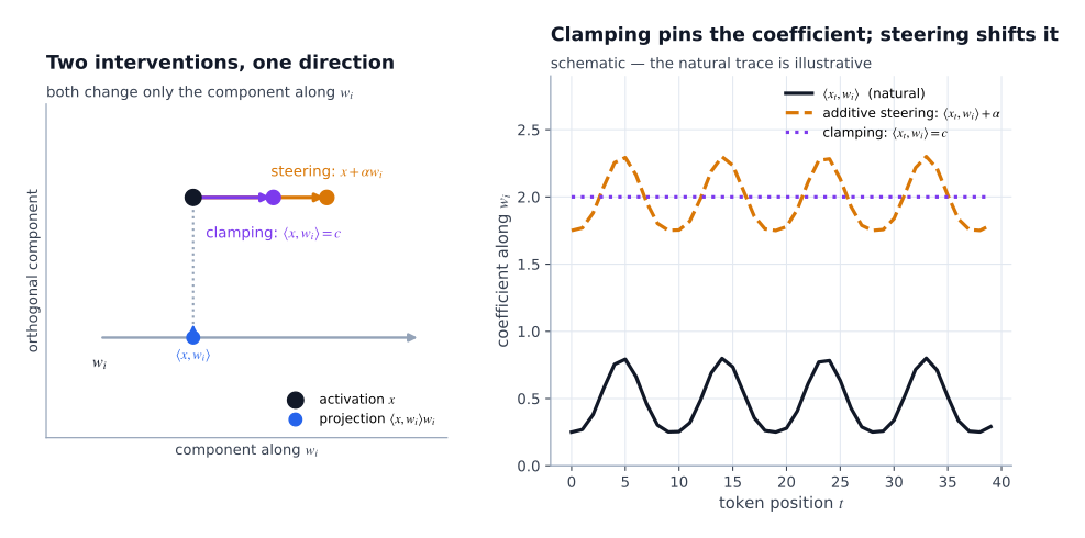
Figure 12.1 — Left: the geometry of the two interventions. Both change only the component of the activation along $w_i$; the orthogonal part of $x$ is untouched. Steering lands at $\langle x,w_i\rangle+\alpha$ and therefore depends on the natural coefficient, while clamping lands at exactly $c$. Right: the same distinction along a sequence of token positions — the natural coefficient fluctuates, so a fixed steering strength is an uneven intervention, whereas clamping is uniform. (The traces are schematic.)
In an SAE-based implementation one often intervenes in the latent space instead: set $f_i(x)\leftarrow c$, leave the other latent coordinates unchanged, and reconstruct,
\[\hat x = b_{\mathrm{pre}}+\sum_{j\neq i}f_j(x)w_j+c\,w_i.\]This is the operation usually meant by feature clamping in SAE interpretability, and it is exactly the latent-space version of the geometric formula above.
12.4 Why clamping can preserve coherence
A large clamp does not force every output token to be “Golden Gate Bridge”. Instead it creates a persistent contextual bias:
\[x_t\longleftarrow x_t-\langle x_t,w_i\rangle w_i+c\,w_i\]at every residual-stream site where the intervention is applied. The model still receives the user prompt, still attends to context, and still applies its normal nonlinear computation. The clamped feature raises the probability of related continuations, but those continuations are selected only when they remain compatible with syntax, discourse coherence, and the rest of the activation pattern.
A useful way to put it:
Clamping does not replace the model’s context; it adds a persistent feature context.
This is why the model may mention the concept frequently, attempt to correct itself when the output becomes implausible, and still remain broadly coherent — and also why the intervention has a dose-response structure: as $c$ grows, the behaviour changes smoothly from “no effect” through “biased” to “degenerate”, and the useful range is a window, not a point.
13. Case Study: The Golden Gate Bridge
13.1 The experiment
Anthropic’s Scaling Monosemanticity (Templeton et al. 2024) identified a Golden Gate Bridge feature in Claude 3 Sonnet, with feature id 34M/31164353. Its strongest activations occurred on references to the bridge, with weaker activations on related landmarks and monuments.
The intervention: clamp this feature to approximately $10\times$ its maximum naturally observed activation during the forward pass. The resulting model — popularly “Golden Gate Claude” — produced coherent text but repeatedly introduced the Golden Gate Bridge into unrelated responses; in some examples it described itself as the bridge.
13.2 What it established
The scientific content is not the humour. It is this: a single learned direction, identified by an SAE, could be mechanically amplified and produce a systematic, interpretable behavioural change, without reducing the model to gibberish. That is a strong result for the causal reading of SAE features, because:
- the feature was found by an unsupervised method (dictionary learning), not by supervised labelling;
- the intervention was surgical — a single direction, with a magnitude and a sign;
- the effect was specific — it produced the concept the feature was hypothesised to represent, not generic noise;
- and it was graded — the effect scaled with the clamp, and degraded at extreme values.
13.3 What it did not
It did not show that the model “contains a Golden Gate Bridge module”. It showed that a direction exists in activation space whose amplification produces bridge-related output. Distinguishing these is exactly the difference between representation and mechanism (Part 2, §10.6), and it is the reason the field treats steering as strong evidence for a feature’s meaning but not as proof of a mechanism.
14. Applications to Alignment and Safety
The same machinery — dictionary learning, then intervention — has been turned on models rather than on features.
14.1 Model diffing with SAEs
Suppose we have two closely related models: a base model $M_0$ and a fine-tuned model $M_1$ (for example, $M_1$ is $M_0$ after fine-tuning on a small dataset of insecure code). Train or reuse an SAE on activations from $M_0$, then compare each feature’s average activation across the two models:
\[\boxed{ \Delta_i = \mathbb E_{x\sim M_1}\bigl[f_i(x)\bigr] - \mathbb E_{x\sim M_0}\bigl[f_i(x)\bigr]. }\]Features with large positive $\Delta_i$ became more active after fine-tuning; features with large negative $\Delta_i$ became less active.
This is called model diffing, and it is powerful because it does not require any labels about what changed — it reports which features changed, and human (or automated) interpretation comes second. The caveat from Part 2 applies with full force: the comparison is only as meaningful as the assumption that the $M_0$-dictionary transfers to $M_1$. If the fine-tuning has substantially reorganised the representation, the same index no longer denotes the same feature, and a large $\Delta_i$ may mean “the feature moved” rather than “the behaviour changed”.
14.2 Emergent misalignment
OpenAI studied emergent misalignment in GPT-4o using SAEs. Fine-tuning on a narrow set of insecure-code examples produced broader misaligned behaviour across unrelated domains. SAE-based model diffing identified persona-like features whose activations changed substantially after fine-tuning.
Two features are worth describing:
- One was interpreted as a broadly helpful, safe assistant persona. Its activation decreased in the misaligned model, suggesting that it had been suppressing undesirable behaviour.
- Another, among the largest positive changes, activated on text involving violence, harm, or malicious behaviour, and was interpreted as a toxic persona feature.
The causal test was steering:
- increasing the toxic-persona direction increased misaligned behaviour;
- decreasing it reduced misaligned behaviour across multiple domains.
The intervention could not be increased indefinitely: at sufficiently large strength, outputs began to degrade, with some fraction becoming gibberish. This is the practical constraint of §12.4 in the wild — steering strength must be chosen inside the window where the model remains functionally coherent.
14.3 Refusal, sycophancy, and unsafe code
SAEs and related activation-analysis methods have been used to identify directions associated with:
- refusal of harmful requests;
- sycophancy or excessive praise;
- unsafe coding practices, including backdoor insertion;
- honesty, secrecy, deception, and other persona-like behaviours.
For a refusal direction $w_{\mathrm{refusal}}$, the natural experiment is
\[x\longleftarrow x-\alpha w_{\mathrm{refusal}}, \qquad \alpha>0,\]suppressing the direction, with the hypothesis that refusal behaviour weakens; and the converse, adding the direction, to strengthen it.
14.4 The dual-use problem
These tools are scientifically useful and security-relevant. In an open-weight model, an adversary who can identify behaviourally relevant directions could use them to weaken safety training — the same intervention that suppresses refusal is available to anyone with the weights. The response so far has been a mix of release decisions about which SAEs to publish, and a norm of releasing the method while being careful with specific directions. This tension is unresolved and is one of the genuinely open questions in the field, not a technicality.
15. The Linear Representation Hypothesis
15.1 The statement
The linear representation hypothesis says that many semantically meaningful relations in a language model are encoded approximately linearly in activation space. A simple instance:
\[v_{\mathrm{queen}}-v_{\mathrm{king}} \;\approx\; v_{\mathrm{woman}}-v_{\mathrm{man}},\]or equivalently
\[v_{\mathrm{king}}-v_{\mathrm{man}} \;\approx\; v_{\mathrm{queen}}-v_{\mathrm{woman}}.\]The shared difference direction can be read as a gender direction. More generally, for a semantic attribute $A$ one hypothesises a direction $u_A$ such that
\[v_{\text{word with }A}-v_{\text{word without }A} \;\approx\; c\,u_A.\]This is the hypothesis that makes “steer along a direction and change a behaviour” coherent: if the attribute is linear in activation space, then it has a direction.
15.2 Word2vec-style structure
In a simple embedding model, a word $w$ is represented by $v_w\in\mathbb R^d$, and co-occurrence is predicted by a softmax over inner products:
\[\mathbb P(c\mid w)\propto\exp(\langle v_w,v_c\rangle).\]Training encourages geometric structure: words appearing in similar contexts receive similar embeddings, and systematic semantic contrasts become approximately parallel differences — the parallelogram
\[v_{\mathrm{king}}-v_{\mathrm{man}} \approx v_{\mathrm{queen}}-v_{\mathrm{woman}}.\]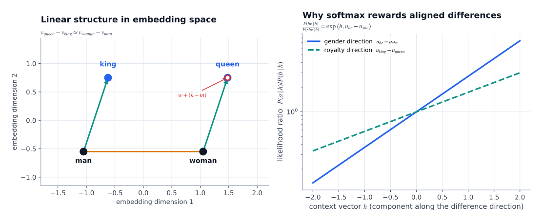
Figure 15.1 — Left: the parallelogram relation. The difference $v_{\mathrm{king}}-v_{\mathrm{man}}$ (teal) and $v_{\mathrm{queen}}-v_{\mathrm{woman}}$ (teal) are approximately parallel and equal in length, so the “gender” direction transfers across the “royalty” contrast. Right: the softmax likelihood ratio for a token pair is $\exp(\langle h, u_a-u_b\rangle)$, so a single linear direction in $h$ controls the ratio — which is what makes aligned unembedding differences useful.
15.3 Why softmax encourages linear contrasts
Consider a model predicting the next token from a residual-stream vector $h\in\mathbb R^d$, with unembedding vectors $u_t$ for tokens $t$:
\[\mathbb P(t\mid h) = \frac{\exp(\langle h,u_t\rangle)} {\sum_s\exp(\langle h,u_s\rangle)}.\]For a token pair $(a,b)$, the likelihood ratio is
\[\frac{\mathbb P(a\mid h)}{\mathbb P(b\mid h)} = \frac{\exp(\langle h,u_a\rangle)}{\exp(\langle h,u_b\rangle)} = \exp\!\left(\langle h,\,u_a-u_b\rangle\right).\]So the entire dependence of the ratio on the context is through the single scalar $\langle h,u_a-u_b\rangle$. Now consider two pairs — $(\text{he},\text{she})$ and $(\text{king},\text{queen})$ — whose likelihoods should respond to the same underlying cue (gender, say), while the context is not independently informative about royalty. A simple way to achieve this is to make the two difference directions align:
\[u_{\mathrm{he}}-u_{\mathrm{she}} \;\approx\; u_{\mathrm{king}}-u_{\mathrm{queen}}.\]Then both ratios depend on $h$ through the same direction, and the model can implement “gender” with a single linear functional of the residual stream. Gradient descent pushes the unembedding differences into such an alignment, and once the unembeddings have this structure, the residual-stream representations are pushed to encode the relevant semantic direction linearly as well.
This is a heuristic, but a useful one: it explains why linear semantic structure appears in both word2vec-style models and transformer language models, and why “king − man + woman ≈ queen” is not a coincidence of culture but a consequence of the softmax likelihood.
15.4 The logit lens
The logit lens interprets an intermediate residual-stream vector $h^{(\ell)}$ by applying the final unembedding matrix at layer $\ell$:
\[\ell_t^{(\ell)}=\langle h^{(\ell)},u_t\rangle,\]and inspecting the tokens with the largest logits:
\[\arg\max_t\,\ell_t^{(\ell)}.\]This provides a provisional reading of what the model is representing at layer $\ell$. It is not ground truth — intermediate representations need not lie in the format that the final layer expects — but it is often informative, and it is a standard sanity check when hunting for features.
A related diagnostic averages the residual-stream vectors over a context,
\[\bar h=\frac1T\sum_{t=1}^T h_t, \qquad \ell_t=\langle\bar h,u_t\rangle.\]In some word-guessing or hidden-word tasks this simple average recovers the intended word with surprisingly high rank. Subtracting a context-mean activation can improve the result further by removing a generic “English definition context” direction.
15.5 Caveats
The linear representation hypothesis is a hypothesis about some relations, not a law:
- It is clearly true for some attribute directions and false for others. Features that are inherently relational or non-linear (§16) are exactly the ones a single direction cannot express.
- Even where it holds, it holds approximately, and the approximation quality varies across the input distribution.
- The hypothesis is about representation, not about mechanism — as in §13.3, a linear direction that predicts behaviour does not by itself tell you the model uses it that way.
16. Feature Manifolds
16.1 Definition
A feature manifold is a low-dimensional nonlinear subset of activation space along which a meaningful semantic variable varies. Formally, if a semantic variable $\theta$ takes values in a parameter space $\Theta$, a feature manifold is a smooth map
\[\Phi:\Theta\to\mathbb R^{d},\]such that activations associated with the value $\theta$ lie near $\Phi(\theta)$.
Typical parameter spaces:
- $\Theta=S^1$: days of the week; months in a cyclic representation;
- $\Theta=\mathbb R^2$: geographic coordinates;
- $\Theta=S^2$: positions on the celestial sphere;
- $\Theta=S^1\times S^1$: products of circular variables.
16.2 Four examples
Geographic structure
Linear probes on activations from a large language model have found representations of countries, continents, and U.S. states whose geometry resembles their real-world geographic arrangement; in such cases, the first two principal components of city-related activations can approximate a map.
Days of the week
Activations associated with days of the week can form an approximate circle in a two-dimensional subspace, with moving along the circle corresponding to changing the day. This suggests a representation of the form
\[\Phi(\theta)=R(\theta)\,\Phi(\theta_0), \qquad \theta\in[0,2\pi),\]where $R(\theta)$ is a rotation.
Modular arithmetic
In small transformers trained to compute modular addition, one finds circular structures in activation space: $a+b\bmod n$ is associated with composing rotations on a circle, and the model implements part of the addition by composing such rotations.
The celestial sphere
One study of questions about locating stars and constellations found that activations could align with the celestial sphere: principal components of the activations reflected actual sky coordinates, and rotating along the recovered spherical manifold could change model answers about stellar location. This example is instructive because the semantic variable is naturally two-dimensional and curved: a point on the sky is a point on a sphere, not on a line.
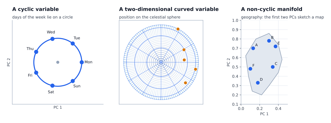
Figure 16.1 — The three shapes of structure a linear dictionary cannot represent directly. Left: a cyclic variable (days of the week) on a circle. Middle: a curved two-dimensional variable (celestial coordinates) on a sphere. Right: a non-cyclic manifold (geography) with no rotational symmetry, whose first two principal components can sketch a map. All three are schematics of the geometry, not measurements.
16.3 Manifold-aware steering
If a concept lives on a manifold, additive steering may be the wrong intervention. If the days of the week lie on a circle, then moving from “Monday” to “Wednesday” should move along the circle:
\[x_{\mathrm{Wednesday}}\approx R(\Delta\theta)\,x_{\mathrm{Monday}}.\]Simply adding a fixed vector may leave the manifold, producing an activation that the model treats as unnatural — and the result is usually worse than doing nothing, because out-of-distructure activations elicit out-of-distribution behaviour.
Manifold-aware steering therefore asks
\[x\longleftarrow\Phi(\theta_{\mathrm{new}})\]rather than
\[x\longleftarrow x+\alpha w_i.\]In practice this requires more than the manifold itself: one may need to model both the tangent direction along the manifold and perturbations in its normal directions, and the map $\Phi$ has to be learned or estimated for the concept in question.
16.4 The general recipe
A workable pipeline for manifold-aware work:
- Suspect a variable. Days of the week, geographic location, modular arithmetic, celestial position — these are the cases where manifolds have been found.
- Find the manifold. Take a large set of activations differing in the suspected variable, project them (PCA, or a random projection followed by a local method), and look for low-dimensional curved structure.
- Learn the parameterisation. Fit a map $\Phi:\Theta\to\mathbb R^d$ (or a local linear model in the tangent space) relating activations to the semantic coordinate.
- Test causally. Move the activation along the manifold and check that the model’s behaviour changes as the variable changes — and only as the variable changes. This is the step that distinguishes a real manifold from a coincidence in the probe.
- Combine with sparse features. A single activation may carry both a sparse linear part and a manifold coordinate; the decomposition should be estimated jointly (next section).
17. Limitations of Sparse Autoencoders
Everything in Parts 2 and 3 rests on SAEs, so it is worth being precise about what they cannot do.
17.1 Dark matter
Even very wide SAEs leave a nonzero reconstruction error:
\[\mathbb E_x\|x-\hat x\|_2^2>0.\]The unexplained component is sometimes called the dark matter of SAEs. It may contain:
- noise;
- nonlinear structure (feature manifolds);
- information not naturally expressible as a sparse linear combination of directions;
- features too rare or too weak for the chosen dictionary width.
17.2 No canonical dictionary
SAE dictionaries are not unique. Different seeds, widths, sparsity levels, architectures, and training datasets produce different feature sets that all reconstruct the activations reasonably well. There is therefore generally no canonical ground-truth decomposition of a residual-stream vector into features.
This is the deepest conceptual weakness: when we say “feature $i$ means $X$”, we mean that this particular learned dictionary contains a direction whose activation pattern and causal effect resemble $X$. The label is about a dictionary element, not about the model.
17.3 Feature splitting and absorption
As $N$ increases, a single feature in a smaller SAE may split into several features in a larger SAE. For example, an “Einstein” feature in a smaller SAE may become, in a larger SAE, several features related to:
- names beginning with “E”;
- galaxies and science;
- scientists;
- prominent German figures.
The reverse happens too: feature absorption, where several related concepts merge into one feature.
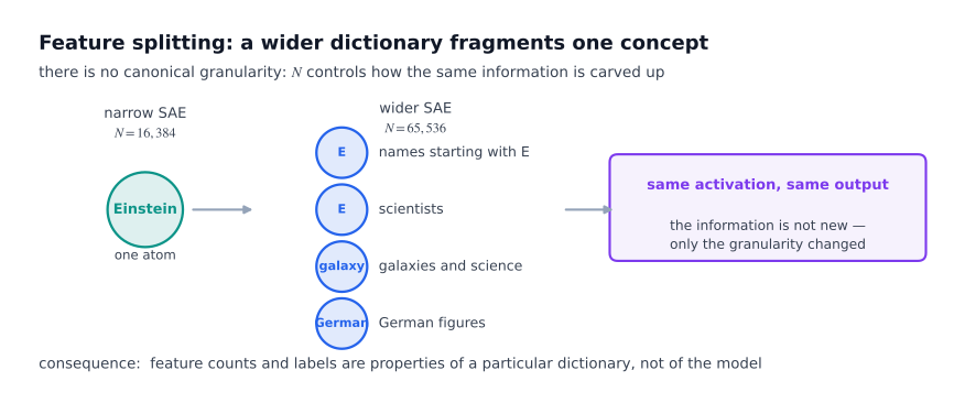
Figure 17.1 — Feature splitting. Increasing the dictionary width can fragment a single concept into several partially overlapping features. The information content is unchanged; only the granularity of the decomposition differs. (Schematic.)
17.4 Hierarchical concepts
Language has hierarchical structure:
\[\text{animal}\supset\text{dog}\supset\text{poodle}.\]One might hope that a wider SAE would first recover broad categories and then refine them into subordinate concepts. In practice the relationship is not so clean: a larger SAE may split a compact concept such as “Einstein” into several partially overlapping features rather than preserving it as one atomic unit and adding finer subconcepts. Increasing $N$ does not necessarily produce more fundamental or more atomic concepts; it may produce a different, more fragmented decomposition.
17.5 Nonlinear structure
SAEs model activations as sparse linear combinations:
\[x\approx b_{\mathrm{pre}}+\sum_i f_i(x)w_i.\]This is powerful, but it is fundamentally a first-order linear approximation. If the activation distribution contains meaningful curved structure — circles, spheres, spirals, tori — a sparse linear dictionary may destroy or obscure it. A circular “day-of-week” manifold may be represented by many linear features rather than by an explicit cyclic variable; the relation between them (their arrangement on a circle) is then only recoverable by an additional step.
17.6 What survives all of this
It is worth stating the case for the method plainly, because the limitations are serious and the method is still valuable:
- SAEs give a hypothesis about the model’s computation that is (a) unsupervised, (b) testable by intervention, and (c) composable with a surprising amount of structure (monosemantic features, steering, model diffing, manifolds).
- The absence of a feature in a given dictionary is weak evidence about the model; the presence of a feature, confirmed causally, is strong evidence.
- The limitations above are mostly statements about granularity and linearity. They tell us what to build next, not that the direction is wrong.
18. Open Problems and the Research Program
18.1 Manifold-aware SAEs
A major open problem is a principled method combining:
- sparse dictionary learning;
- nonlinear manifold discovery;
- causal validation.
One possible target is an SAE-like model whose latent variables include both sparse linear features and low-dimensional manifold coordinates:
\[x \approx b_{\mathrm{pre}} + \sum_{i=1}^{N} f_i(x)w_i + \Phi\bigl(\theta(x)\bigr),\]where $f_i(x)$ are sparse linear feature activations, $w_i$ the linear dictionary directions, $\theta(x)\in\Theta$ a low-dimensional manifold coordinate, and $\Phi:\Theta\to\mathbb R^d$ a learned nonlinear embedding.
18.2 Unsupervised manifold discovery
Current feature-manifold examples are usually found after suspecting the relevant variable — days of the week, geographic location, modular arithmetic, celestial position. A major advance would be a method that analyses activations without knowing the target concept and discovers a meaningful nonlinear object automatically. Formally: given activations ${x_1,\dots,x_n}\subseteq\mathbb R^d$, find a low-dimensional manifold $\mathcal M\subseteq\mathbb R^d$ and a semantic parameterisation $\Phi:\Theta\to\mathcal M$ such that variation along $\mathcal M$ corresponds to a causally meaningful model variable.
18.3 Better evaluation
SAE evaluation should not rest on reconstruction error and sparsity alone. Useful criteria include:
- causal behavioural effects;
- robustness across prompts and contexts;
- stability across random seeds;
- compositional consistency;
- preservation of downstream model performance;
- ability to support precise interventions;
- relationship to human-interpretable concepts.
18.4 The program
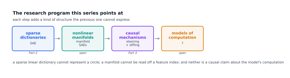
Figure 18.1 — The research program this series points at: sparse dictionaries (Part 2) → nonlinear manifolds (open) → causal mechanisms (Part 3) → models of computation (open). Each step adds a kind of structure the previous one cannot express.
\[\text{linear features} \longrightarrow \text{sparse dictionaries} \longrightarrow \text{nonlinear manifolds} \longrightarrow \text{causal models of computation}.\]SAEs are a powerful first-order tool, but they are not yet a complete theory of neural representation. The field is searching for representations that are simultaneously sparse, interpretable, causally validated, stable across scales, and capable of representing nonlinear and hierarchical structure.
18.5 Part 3 Takeaways
- Correlation is not mechanism. Additive steering ($x\mapsto x+\alpha w_i$) and feature clamping ($x\mapsto x+(c-\langle x,w_i\rangle)w_i$) are the two interventions; the second sets the coefficient, the first shifts it, and both are graded — there is a window of useful strength, not a point.
- Clamping a Golden Gate Bridge feature to ~10× its maximum produced coherent but bridge-obsessed behaviour: strong evidence that SAE directions have systematic causal meaning, not proof of a “bridge module”.
- Model diffing ($\Delta_i=\mathbb E_{M_1}[f_i]-\mathbb E_{M_0}[f_i]$) finds what changed after fine-tuning without labels; the GPT-4o emergent-misalignment work used it to find a “toxic persona” feature whose causal role was then confirmed by steering.
- The same methods are dual-use: a direction that suppresses refusal is available to anyone with the weights.
- The linear representation hypothesis ($v_{\mathrm{queen}}-v_{\mathrm{king}}\approx v_{\mathrm{woman}}-v_{\mathrm{man}}$) has a mechanism: the softmax likelihood ratio is $\exp(\langle h,u_a-u_b\rangle)$, so aligned unembedding differences let one linear functional of $h$ control several token contrasts.
- Feature manifolds — circles for days of the week, maps for geography, spheres for the sky — are the structures a sparse linear dictionary cannot express, and they call for interventions that move along a manifold rather than along a fixed direction.
- SAEs are incomplete: they leave dark matter, have no canonical dictionary, split and absorb concepts, handle hierarchy poorly, and flatten nonlinear structure.
- The open problems are concrete: joint sparse + manifold models, unsupervised manifold discovery, and evaluation criteria that are causal rather than reconstructive.
19. The Series Bibliography
Compressed sensing and high-dimensional geometry
- E. J. Candès and T. Tao. Decoding by linear programming. IEEE Transactions on Information Theory, 51(12):4203–4215, 2005.
- E. J. Candès, J. Romberg, and T. Tao. Robust uncertainty principles: exact signal reconstruction from highly incomplete frequency information. IEEE Transactions on Information Theory, 52(2):489–509, 2006.
- E. J. Candès. The restricted isometry property and its implications for compressed sensing. Comptes Rendus Mathématique, 346(9–10):589–592, 2008. Exact-recovery threshold: $\delta_{2s}<\sqrt2-1$.
- E. J. Candès, Y. Eldar, D. Mixon, and S. Vempala. An Introduction to Compressed Sensing. Foundations and Trends in Signal Processing, 6(1–4):1–142, 2011.
- R. G. Baraniuk, M. A. Davenport, R. A. DeVore, and M. B. Wakin. A simple proof of the restricted isometry property for random matrices. Constructive Approximation, 28(3):253–263, 2008.
- R. Vershynin. High-Dimensional Probability: An Introduction with Applications in Data Science. Cambridge University Press, 2018. Spherical cap bounds, concentration on the sphere, RIP for sub-Gaussian matrices.
- J. Matoušek. Lectures on Discrete Geometry. Springer, 2002. Spherical caps, coverings and packings.
- S. Boyd. Combinatorial Optimization. Cambridge University Press, 2004. Linear programming duality, basis pursuit, $\ell_1$ vs. $\ell_0$.
- R. Tibshirani. Regression shrinkage and selection via the Lasso. Journal of the Royal Statistical Society B, 58(1):267–288, 1996.
Sparse autoencoders and superposition
- A. Bricken, A. Templeton, J. Batson, B. Chen, A. Jermyn, T. Conerly, et al. Towards monosemanticity: decomposing language models with dictionary learning. Transformer Circuits Thread, 2023.
- H. Cunningham, A. Ewart, L. Riggs, R. Huben, and L. Sharkey. Sparse autoencoders find highly interpretable features in language models. ICLR, 2024. arXiv:2309.08600.
- A. Templeton, T. Conerly, J. Marcus, J. Lindsey, T. Bricken, B. Chen, et al. Scaling monosemanticity: extracting interpretable features from Claude 3 Sonnet. Transformer Circuits Thread, 2024.
- L. Gao, T. Dupré la Tour, H. Tillman, G. Goh, R. Troll, A. Radford, I. Sutskever, J. Leike, and J. Wu. Scaling and evaluating sparse autoencoders. arXiv:2406.04093, 2024.
- S. Rajamanoharan, T. Conerly, A. Jermyn, N. Nanda, J. Leike, and T. Bricken. Jumping ahead: improving reconstruction fidelity with JumpReLU sparse autoencoders. arXiv:2407.14435, 2024.
- B. Bussmann, P. Leask, and N. Nanda. Learning multi-level features with Matryoshka sparse autoencoders. ICML, 2025. arXiv:2503.17547.
- T. Lieberum, S. Rajamanoharan, A. Conmy, L. Smith, N. Nanda, et al. Gemma Scope: open sparse autoencoders everywhere all at once on Gemma 2. arXiv:2408.05147, 2024.
- N. Elhage, T. Hume, C. Olsson, N. Schiefer, T. Henighan, S. Kravec, et al. Toy models of superposition. Transformer Circuits Thread, 2022. arXiv:2209.10652.
- E. J. Mairal, P. Calandrino, and J. Ponce. Online dictionary learning for sparse coding. ECCV, 2010. (MOD.)
- A. M. Bruckstein, D. Donoho, and M. Elad. Sparse solutions for underdetermined systems of linear equations. IEEE Transactions on Information Theory, 42(2):407–425, 1996. (Sparse coding.)
- M. Aharon and M. Elad. Sparse and redundant representation modeling: dictionary learning. (Gated SAE / LASSO dictionary learning.)
- A. Conmy, et al. Scaling up the evaluation of sparse autoencoders. 2023. Standard evaluation battery: $L_0$, FVE, downstream cross-entropy increase.
Interpretation, steering, and safety
- G. Billis, S. Marks, J. Bricken, et al. Language models can explain neurons in language models. OpenAI, 2023. (Simulation, detection, fuzzing.)
- G. Paulo, A. Mallen, C. Juang, and N. Belrose. Automatically interpreting millions of features in large language models. 2024.
- N. Boulyrikov, et al. Activation patching: a technique for attributing behaviour to internal components. (2023.) See also: the broader “causal scrubbing” methodology.
- OpenAI. Emergent misalignment research paper. 2024. SAE-based model diffing on GPT-4o; persona features; steering as the causal test.
- N. Elhage, et al. Discovering and manipulating (or ‘steering’) interpretable features in language models. Transformer Circuits Thread, 2022. See also the wider “steering” and “activation addition” literature.
Representation geometry, manifolds, and tools
- N. Elhage, et al. Linearly mapping from image to text. Transformer Circuits Thread, 2021. See also the “linearly structured representation” line of work.
- A. Radford, et al. Language models are few-shot learners. NeurIPS, 2020. (Logit-lens-style reading of intermediate layers; the Language Models are Few-Shot Learners and Interpretability threads.)
- E. Smith, et al. Understanding and predicting abstractions in LLMs. (Feature-space geometry and abstraction directions.)
- T. Bricken, et al. and the emergent world representations line of work (Johnston et al. 2023): internal maps of geography and other structure in GPT-2’s residual stream.
- G. Gurnee and M. Tegmark. Language models represent space and time. ICLR, 2024. (Low-dimensional structure in LLM activations, including periodic variables.)
- J. Nanda, et al. Understanding addition in transformers. (Emergent structure implementing modular addition.)
How to cite this article
BibTeX.
@misc{kumar2026geometry3,
  author       = {Kumar, Ajeet},
  title        = {Geometry of Neural Activations, Part 3: Steering, Linear Structure, and Feature Manifolds},
  year         = {2026},
  orcid        = {\url{https://orcid.org/0009-0001-6494-4217}},
  howpublished = {\url{https://ajeetkbhardwaj.github.io/posts/2026/10/geometry-of-neural-activation-part-3/}},
  note         = {Part 3 of Geometry of Neural Activations}
}

Comments