ddglearn - Discrete Differential Geometry and Its Applications
Published:
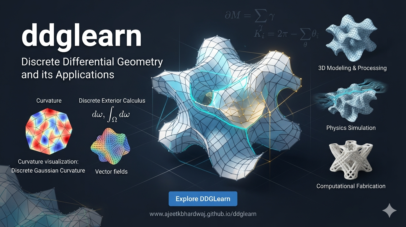
Discrete Differential Geometry studies geometric ideas—curvature, normals, geodesics, and surface deformation—using finite structures such as meshes rather than smooth mathematical surfaces. ddglearn is designed to make these ideas practical: users can load a mesh, compute geometric quantities, experiment with algorithms, and visualize the result.
Why discrete geometry?
In classical differential geometry, a surface is often described as a smooth function with derivatives defined everywhere. Real-world geometry is different: 3D scans, simulations, graphics models, and medical surfaces are usually stored as discrete samples.
A triangle mesh approximates a smooth surface using:
- Vertices: points in 3D space.
- Edges: straight-line connections between vertices.
- Faces: usually triangles formed by three vertices.
- Connectivity: information describing which vertices and edges belong to which faces.
The central idea of DDG is to redefine smooth concepts—such as tangent vectors, curvature, and integration—so that they remain meaningful on these finite structures.
flowchart LR
    A[Smooth surface] --> B[Sample points]
    B --> C[Connect samples]
    C --> D[Triangle mesh]
    D --> E[Discrete geometry]
    E --> F[Curvature, normals, geodesics]
Core data structure: the mesh
Most DDG algorithms begin with a mesh. A mesh is not only a collection of 3D coordinates; its connectivity determines the local neighborhood of every vertex.
For example, to compute curvature at a vertex, the algorithm needs to know:
- Which faces touch the vertex.
- Which vertices are its neighbors.
- The angles and areas of the surrounding triangles.
- The directions of the incident edges.
flowchart TD
    V[Vertex positions] --> M[Mesh]
    F[Face connectivity] --> M
    E[Edge connectivity] --> M
    M --> N[Vertex neighborhood]
    N --> G[Geometric quantities]
    G --> C[Curvature]
    G --> Nv[Normals]
    G --> L[Laplacian]
    G --> P[Geodesics]
A useful mental model is that geometry lives in the vertex positions, while topology lives in the connectivity. Changing vertex positions changes the shape; changing connectivity changes the combinatorial structure of the surface.
From mesh to differential operators
A major strength of DDG is that it converts geometric questions into matrix computations. For a mesh with $n$ vertices, many operators become sparse $n \times n$ matrices.
Common operators include:
| Concept | Discrete version | Typical use |
|---|---|---|
| Gradient | Per-face or per-edge gradient | Transport quantities across a surface |
| Divergence | Area-weighted divergence at vertices | Solve Poisson problems |
| Laplacian | Mesh Laplace-Beltrami operator | Smoothing, spectral analysis, heat flow |
| Curvature | Angle defect, mean curvature, Gaussian curvature | Shape analysis |
| Cotangent weights | Edge weights based on opposite angles | Accurate discrete operators |
flowchart LR
    M[Mesh] --> A[Adjacency]
    M --> W[Cotangent weights]
    M --> Ar[Vertex areas]
    A --> L[Laplace-Beltrami operator]
    W --> L
    Ar --> L
    L --> S[Spectral analysis]
    L --> H[Heat diffusion]
    L --> SM[Mesh smoothing]
The Laplace-Beltrami operator is especially important. Intuitively, it measures how a value at a vertex compares with the values at nearby vertices. If a vertex has a much larger value than its neighbors, the Laplacian is negative; if it is smaller, the Laplacian is positive.
Normals and local orientation
Normals describe the direction perpendicular to a surface at a point. They are essential for rendering, shading, physical simulation, and defining orientation.
For a triangular face with vertices $v_0$, $v_1$, and $v_2$, a normal can be computed from the cross product of two edge vectors:
\[n_f = \frac{(v_1 - v_0) \times (v_2 - v_0)}{\lVert (v_1 - v_0) \times (v_2 - v_0) \rVert}\]A vertex normal is commonly computed as an area-weighted average of the normals of adjacent faces.
flowchart LR
    F[Triangle face] --> CP[Cross product of edges]
    CP --> FN[Face normal]
    FN --> WA[Area-weighted average]
    VA[Adjacent faces] --> WA
    WA --> VN[Vertex normal]
Consistent face orientation matters. If one triangle is wound clockwise and its neighbor counterclockwise, their normals may point in opposite directions, producing incorrect shading, broken boundary detection, or unreliable geometric computations.
Curvature: how a surface bends
Curvature measures how strongly a surface bends. On a smooth surface, curvature is defined using derivatives; on a mesh, it is estimated from local geometry.
Two important types are:
- Gaussian curvature: the product of the two principal curvatures; it describes intrinsic bending.
- Mean curvature: the average of the two principal curvatures; it is often used in smoothing and surface fairing.
A simple discrete estimate of Gaussian curvature at an interior vertex uses the angle defect:
\[K(v) = \frac{2\pi - \sum_i \theta_i}{A(v)}\]Here, $\theta_i$ are the angles at vertex $v$ in its incident triangles, and $A(v)$ is the barycentric or mixed area associated with the vertex.
flowchart TD
    V[Vertex v] --> T[Incident triangles]
    T --> Ang[Angles at v]
    Ang --> Sum[Sum of angles]
    Sum --> Defect[Angle defect]
    Defect --> K[Gaussian curvature]
    T --> Area[Mixed area]
    Area --> K
Interpretation:
- A flat vertex has an angle sum close to $2\pi$, so curvature is near zero.
- A cone-like vertex has an angle sum less than $2\pi$, giving positive curvature.
- A saddle-like vertex can have an angle sum greater than $2\pi$, giving negative curvature.
Geodesics: shortest paths on surfaces
A geodesic is the shortest path between two points constrained to remain on a surface. On a plane, it is a straight line; on a sphere, it resembles a great-circle route.
Computing geodesics is useful for:
- Texture generation.
- Path planning on 3D surfaces.
- Measuring distances on anatomical models.
- Segmenting meshes.
- Analyzing shapes independently of their embedding in 3D space.
flowchart LR
    S[Source vertex] --> H[Initial distance field]
    H --> P[Propagation across mesh]
    P --> U[Distance to every vertex]
    U --> G[Geodesic path]
    T[Target vertex] --> G
A common approach is to compute a distance field from a source vertex, then trace a path backward from the target by following decreasing distance values.
Heat-based geometry
Heat methods provide an elegant way to compute distances and solve PDEs on surfaces. The idea is to release heat at a source and observe how it spreads over the mesh.
The heat equation is:
\[\frac{\partial u}{\partial t} = \Delta u\]On a mesh, this becomes a sparse linear system involving the Laplace-Beltrami operator. After solving for the heat distribution, its gradient can be normalized and used to recover a vector field, from which distances can be computed.
flowchart TD
    S[Heat source] --> H0[Initial heat distribution]
    H0 --> HE[Solve heat equation]
    HE --> HF[Heat field]
    HF --> GR[Gradient of heat field]
    GR --> NV[Normalize vector field]
    NV --> DIV[Compute divergence]
    DIV --> POI[Solve Poisson equation]
    POI --> D[Geodesic distance field]
This workflow is powerful because it avoids explicitly tracing every possible path across the mesh.
Smoothing and denoising
Real meshes often contain noise from scanning, reconstruction, or simulation. Smoothing reduces high-frequency irregularities while trying to preserve important features such as edges and corners.
A basic Laplacian smoothing update moves each vertex toward the average of its neighbors:
\[v_i^{new} = v_i + \lambda \Delta v_i\]where $\lambda$ controls the strength of smoothing.
flowchart LR
    N[Noisy mesh] --> L[Laplacian]
    L --> D[Displacement field]
    D --> U[Update vertex positions]
    U --> S[Smoothed mesh]
    S --> Q{Feature preserved?}
    Q -- No --> C[Adjust smoothing strength]
    C --> L
    Q -- Yes --> F[Final mesh]
Strong smoothing can remove noise but may also erase sharp features. More advanced methods use curvature flow, feature preservation, or optimization-based fairing.
Typical ddglearn workflow
A typical workflow in a DDG library follows this sequence:
flowchart TD
    A[Load mesh] --> B[Validate geometry]
    B --> C[Build adjacency]
    C --> D[Compute areas and normals]
    D --> E[Construct operators]
    E --> F{Choose analysis}
    F --> G[Curvature]
    F --> H[Geodesics]
    F --> I[Smoothing]
    F --> J[Heat diffusion]
    G --> K[Visualize results]
    H --> K
    I --> K
    J --> K
Conceptually, the library can be organized into layers:
flowchart TD
    subgraph Input
        IO[Mesh I/O]
        VAL[Validation]
    end

    subgraph Core
        MESH[Mesh data structure]
        ADJ[Adjacency and neighborhoods]
        OP[Differential operators]
    end

    subgraph Algorithms
        CURV[Curvature]
        GEO[Geodesics]
        SMOOTH[Smoothing]
        HEAT[Heat methods]
    end

    subgraph Output
        VIZ[Visualization]
        EXP[Export results]
    end

    IO --> VAL --> MESH
    MESH --> ADJ --> OP
    OP --> CURV
    OP --> GEO
    OP --> SMOOTH
    OP --> HEAT
    CURV --> VIZ
    GEO --> VIZ
    SMOOTH --> VIZ
    HEAT --> VIZ
    VIZ --> EXP
Example conceptual API
The following pseudocode illustrates the kind of workflow a learning-oriented DDG library might expose:
mesh = ddglearn.load_mesh("surface.obj")

mesh.compute_normals()
mesh.compute_vertex_areas()

curvature = ddglearn.gaussian_curvature(mesh)
laplacian = ddglearn.laplace_beltrami(mesh)

smoothed = ddglearn.smooth(mesh, strength=0.3)
distance = ddglearn.geodesic_distance(mesh, source_vertex=0)

ddglearn.visualize(mesh, scalar_field=curvature)
The important design principle is separation of concerns:
- Mesh representation stores geometry and topology.
- Operators translate geometry into matrices and local computations.
- Algorithms combine operators to solve high-level problems.
- Visualization makes the result interpretable.
Applications
DDG appears across many technical domains:
| Domain | How DDG is used |
|---|---|
| Computer graphics | Mesh editing, shading, deformation, remeshing |
| Physical simulation | Cloth, shells, fluids, and elastic surfaces |
| 3D scanning | Denoising, hole filling, surface reconstruction |
| Medical imaging | Organ shape analysis and anatomical measurements |
| Architecture | Structural surface analysis and form-finding |
| Machine learning | Geometric deep learning and mesh-based neural networks |
Conclusion
ddglearn can serve as both a practical geometry toolkit and a learning environment. By exposing meshes, differential operators, curvature, geodesics, and heat-based methods through code, it helps users move beyond formulas and see how geometric ideas behave on real 3D data.
Comments